Count Models: Understanding the Log Link Function

When we run a statistical model, we are in a sense creating a mathematical equation. The simplest regression model looks like this:

Y_i = β₀ + β₁X+ ε_i

The left side of the equation is the sum of two parts on the right: the fixed component, β₀ + β₁X, and the random component, ε_i.

You’ll also sometimes see the equation written about the mean or expected value of Y on the left and only the fixed component on the right:

μ_Y|X = β₀ + β₁X

All we’ve done is remove that random component from both sides to focus on the fixed portion. Why?

The random component has a probability distribution. Since the outcome variable Y includes that random component, it too follows a probability distribution.

In linear regression, we assume that probability distribution is normal.  But there are a lot of outcome variables for which a normal distribution doesn’t fit.

Generalized Linear Models

Generalized linear models allow a few other distributions, including Poisson, binomial, and Gamma (among others).

But in order to make the model fit in a linear form for these other distributions, we often need to take some function of the mean. That second equation above doesn’t fit.

In generalized linear models, there is a link function, which is the link between the mean of Y on the left and the fixed component on the right.

f(μ_Y|X) = β₀ + β₁X

It’s very possible you have run models without being aware of this. Some software packages have models (e.g., Stata’s nbreg or SAS proc logistic) that use a default link function.

But if you run a generalized linear model in a more general software procedure (like SAS’s proc genmod or R’s glm), then you must select the link function that works with the distribution in the random components.

A natural fit for count variables that follow the Poisson or negative binomial distribution is the log link. The log link exponentiates the linear predictors. It does not log transform the outcome variable.

Here are two versions of the same basic model equation for count data:

ln(μ) = β₀ + β₁X

μ = exp(β₀ + β₁X), also written as μ = e^{β₀ + β₁X}

Where μ=predicted value of Y given X, exp(β₀) = the effect on the mean of μ when X=0, and exp(β₁)= the multiplicative effect on the mean of Y for a one-unit increase in X.  e is a constant value of approximately 2.72.

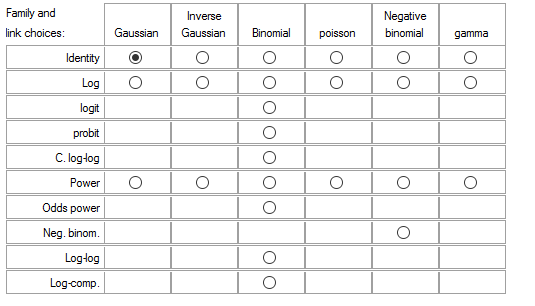
There are several link choices for each probability distribution. The table below shows the potential combinations allowed in Stata.

But there is generally a best fitting link for each distribution, the canonical link. Be sure to choose the best fit.

**This article was updated Nov. 12th, 2020.

Jeff Meyer is a statistical consultant with The Analysis Factor, a stats mentor for Statistically Speaking membership, and a workshop instructor. Read more about Jeff here.

Poisson and Negative Binomial Regression for Count Data

Learn when you need to use Poisson or Negative Binomial Regression in your analysis, how to interpret the results, and how they differ from similar models.

Take Me to The Video!