Generalized Linear Models in R, Part 7: Checking for Overdispersion in Count Regression

In my last blog post we fitted a generalized linear model to count data using a Poisson error structure.

We found, however, that there was over-dispersion in the data – the variance was larger than the mean in our dependent variable.

Over-dispersion is a problem if the conditional variance (residual variance) is larger than the conditional mean.  One way to check for and deal with over-dispersion is to run a quasi-poisson model, which fits an extra dispersion parameter to account for that extra variance.

Now let’s fit a quasi-Poisson model to the same data.

model2 <- glm(Students ~ Days, quasipoisson) summary(model2) Call: glm(formula = Students ~ Days, family = quasipoisson) Deviance Residuals: Min 1Q Median 3Q Max -2.00482 -0.85719 -0.09331 0.63969 1.73696 Coefficients: Estimate Std. Error t value Pr(>|t|)    
(Intercept)  1.990235   0.074789   26.61   <2e-16 ***
Days        -0.017463   0.001539  -11.35   <2e-16 ***
---
Signif. codes:  0 ‘***’ 0.001 ‘**’ 0.01 ‘*’ 0.05 ‘.’ 0.1 ‘ ’ 1

(Dispersion parameter for quasipoisson family taken to be 0.7939441)

    Null deviance: 215.36  on 108  degrees of freedom
Residual deviance: 101.17  on 107  degrees of freedom
AIC: NA

Number of Fisher Scoring iterations: 5

The outcome of our attempt to account for over-dispersion is that the residual deviance has not changed.

The dispersion parameter, which was forced to be 1 in our last model, is allowed to be estimated here. In fact, it is estimated at .79.

This parameter tells us how many times larger the variance is than the mean. Since our dispersion was less than one, it turns out the conditional variance is actually smaller than the conditional mean. We have under-dispersion, not over.

We can extract the model coefficients in the usual way:

model2$coefficients  
(Intercept)     Days 
 1.99023497 -0.01746317

Anyway – we now plot the regression. We set up a time axis running from 0 to 150 (the number of days). However, we include small increments of 0.1 in order to create a smooth appearance to our plot. We will evaluate the model on these values and then use those values to plot the model.

timeaxis <-seq 0="" 150="" 1="" pre="">

Anyway – we now plot the regression. We set up a time axis running from 0 to 150 (the number of days). However, we include small increments of 0.1 in order to create a smooth appearance to our plot. We will evaluate the model on these values and then use those values to plot the model.

timeaxis <-seq (0,150,0.1)

Now we use the predict() function to set up the fitted model values.

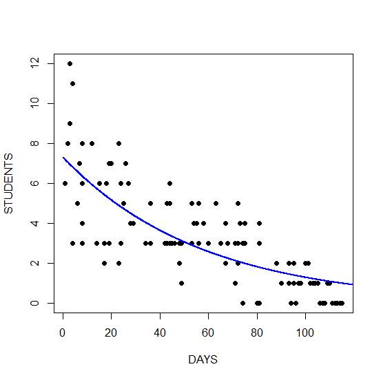
Y <- predict(model2, list(Days = timeaxis))

plot(Days, Number, xlab = "DAYS", ylab = "STUDENTS", pch = 16)

Finally, we plot the fitted model. We take the exponential of the fitted values because the fitted values are returned on a logarithmic scale. Taking the exponential back-transforms from the log scale to the original data.

lines(timeaxis, exp(Y), lwd = 2, col = "blue")

The graph shows a non-linear decrease in cases with number of days. Of course, instead of taking the exponential of the fitted values, we could also have used the predict() function together with the argument type = “response”.

Z <- predict(model2, list(Days = timeaxis), type = "response")

plot(Days, Number, xlab = "DAYS", ylab = "NUMBER", pch = 16)

lines(timeaxis, Z, lwd = 2, col = "red")

Let’s calculate the impact on the number of cases arising from a one day increase along the time axis. First we take the exponential of the coefficients.

coeffs <- exp(coef(model2))

coeffs
(Intercept)        Days 
  7.3172529   0.9826884

We calculate the 95% confidence interval (upper and lower confidence limits) as follows:

CI <- exp(confint.default(model2))

CI
              2.5 %    97.5 %
(Intercept) 6.3195674 8.4724454
Days        0.9797296 0.9856562

We can calculate the change in number of students presenting with the disease for each additional day, as follows:

1 - 0.9826884
[1] 0.0173116

The reduction (rate ratio) is approximately 0.02 cases for each additional day.

****

See our full R Tutorial Series and other blog posts regarding R programming.

About the Author: David Lillis has taught R to many researchers and statisticians. His company, Sigma Statistics and Research Limited, provides both on-line instruction and face-to-face workshops on R, and coding services in R. David holds a doctorate in applied statistics.

Poisson and Negative Binomial Regression for Count Data

Learn when you need to use Poisson or Negative Binomial Regression in your analysis, how to interpret the results, and how they differ from similar models.

Take Me to The Video!