 Last time we created two variables and used the lm() command to perform a least squares regression on them, and diagnosing our regression using the plot() command.
Just as we did last time, we perform the regression using lm(). This time we store it as an object M.
M <- lm(formula = height ~ bodymass)
Now we use the summary() command to obtain useful information about our regression:
summary(M)
Call:
lm(formula = height ~ bodymass)

Residuals:
   Min     1Q Median     3Q     Max
-10.786 -8.307   1.272   7.818 12.253

Coefficients:
           Estimate Std. Error t value Pr(>|t|)
(Intercept) 98.0054   11.7053   8.373 3.14e-05 ***
bodymass     0.9528     0.1618   5.889 0.000366 ***
---
Signif. codes: 0 ‘***’ 0.001 ‘**’ 0.01 ‘*’ 0.05 ‘.’ 0.1 ‘ ’ 1

Residual standard error: 9.358 on 8 degrees of freedom
Multiple R-squared: 0.8126,     Adjusted R-squared: 0.7891
F-statistic: 34.68 on 1 and 8 DF, p-value: 0.0003662
Our model p-value is very significant (approximately 0.0004) and we have very good explanatory power (over 81% of the variability in height is explained by body mass). Our diagnostic plots were as follows:
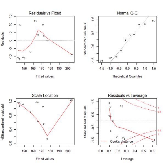
We saw that points 2, 4, 5 and 6 have great influence on the model. Now we see how to re-fit our model while omitting one datum. Let’s omit point 6. Note the syntax we use to do so, involving the subset() command inside the lm() command and omitting the point using the syntax != which stands for “not equal to”. The syntax instructs R to fit a linear model on a subset of the data in which all points are included except the sixth point.
M2 <- lm(height ~ bodymass, subset=(1:length(height)!=6))
summary(M2)
Call:
lm(formula = height ~ bodymass, subset = (1:length(height) !=
    6))
Residuals:
   Min     1Q Median     3Q    Max
-9.331 -7.526  1.180  4.705 10.964

Coefficients:
            Estimate Std. Error t value Pr(>|t|)
(Intercept)  96.3587    10.9787   8.777 5.02e-05 ***
bodymass      0.9568     0.1510   6.337  0.00039 ***
---
Signif. codes:  0 ‘***’ 0.001 ‘**’ 0.01 ‘*’ 0.05 ‘.’ 0.1 ‘ ’ 1
Residual standard error: 8.732 on 7 degrees of freedom
Multiple R-squared: 0.8516,     Adjusted R-squared: 0.8304
F-statistic: 40.16 on 1 and 7 DF,  p-value: 0.0003899
Because we have omitted one observation, we have lost one degree of freedom (from 8 to 7) but our model has greater explanatory power (i.e. the Multiple R-Squared has increased from 0.81 to 0.85). From that perspective, our model has improved, but of course, point 6 may well be a valid observation, and perhaps should be retained. Whether you omit or retain such data is a matter of judgement.
The next post will begin a series of four blogs focused on making generalized linear models in R.
About the Author: David Lillis has taught R to many researchers and statisticians. His company, Sigma Statistics and Research Limited, provides both on-line instruction and face-to-face workshops on R, and coding services in R. David holds a doctorate in applied statistics.
See our full R Tutorial Series and other blog posts regarding R programming.

Leave a Reply