The practice of choosing predictors for a regression model, called model building, is an area of real craft.
There are many possible strategies and approaches and they all work well in some situations. Every one of them requires making a lot of decisions along the way. As you make decisions, one danger to look out for is overfitting—creating a model that is too complex for the the data. (more…)
In a recent article, we reviewed the impact of removing the intercept from a regression model when the predictor variable is categorical. This month we’re going to talk about removing the intercept when the predictor variable is continuous.
Spoiler alert: You should never remove the intercept when a predictor variable is continuous.
Here’s why. (more…)
Predictor variables in statistical models can be treated as either continuous or categorical.
Usually, this is a very straightforward decision.
Categorical predictors, like treatment group, marital status, or highest educational degree should be specified as categorical.
Likewise, continuous predictors, like age, systolic blood pressure, or percentage of ground cover should be specified as continuous.
But there are numerical predictors that aren’t continuous. And these can sometimes make sense to treat as continuous and sometimes make sense as categorical.
(more…)
In the last post, we examined how to use the same sample when running a set of regression models with different predictors.
Adding a predictor with missing data causes cases that had been included in previous models to be dropped from the new model.
Using different samples in different models can lead to very different conclusions when interpreting results.
Let’s look at how to investigate the effect of the missing data on the regression models in Stata.
The coefficient for the variable “frequent religious attendance” was negative 58 in model 3 and then rose to a positive 6 in model 4 when income was included. Results (more…)
An “estimation command” in Stata is a generic term used for a command that runs a statistical model. Examples are regress, ANOVA, Poisson, logit, and mixed.
Stata has more than 100 estimation commands.
Creating the “best” model requires trying alternative models. There are a number of different model building approaches, but regardless of the strategy you take, you’re going to need to compare them.
Running all these models can generate a fair amount of output to compare and contrast. How can you view and keep track of all of the results?
You could scroll through the results window on your screen. But this method makes it difficult to compare differences.
You could copy and paste the results into a Word document or spreadsheet. Or better yet use the “esttab” command to output your results. But both of these require a number of time consuming steps.
But Stata makes it easy: my suggestion is to use the post-estimation command “estimates”.
What is a post-estimation command? A post-estimation command analyzes the stored results of an estimation command (regress, ANOVA, etc).
As long as you give each model a different name you can store countless results (Stata stores the results as temp files). You can then use post-estimation commands to dig deeper into the results of that specific estimation.
Here is an example. I will run four regression models to examine the impact several factors have on one’s mental health (Mental Composite Score). I will then store the results of each one.
regress MCS weeks_unemployed i.marital_status
estimates store model_1
regress MCS weeks_unemployed i.marital_status kids_in_house
estimates store model_2
regress MCS weeks_unemployed i.marital_status kids_in_house religious_attend
estimates store model_3
regress MCS weeks_unemployed i.marital_status kids_in_house religious_attend income
estimates store model_4
To view the results of the four models in one table my code can be as simple as:
estimates table model_1 model_2 model_3 model_4
But I want to format it so I use the following:
estimates table model_1 model_2 model_3 model_4, varlabel varwidth(25) b(%6.3f) /// star(0.05 0.01 0.001) stats(N r2_a)
Here are my results:
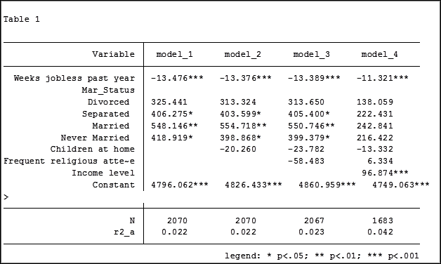
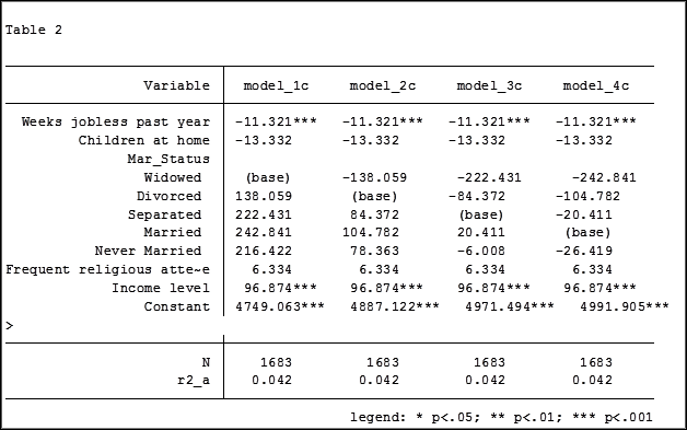
My base category for marital status was “widowed”. Is “widowed” the base category I want to use in my final analysis? I can easily re-run model 4, using a different reference group base category each time.
Putting the results into one table will make it easier for me to determine which category to use as the base.
Note in table 1 the size of the samples have changed from model 2 (2,070) to model 3 (2,067) to model 4 (1,682). In the next article we will explore how to use post-estimation data to use the same sample for each model.
Jeff Meyer is a statistical consultant with The Analysis Factor, a stats mentor for Statistically Speaking membership, and a workshop instructor. Read more about Jeff here.
In a Regression model, should you drop interaction terms if they’re not significant?
In an ANOVA, adding interaction terms still leaves the main effects as main effects. That is, as long as the data are balanced, the main effects and the interactions are independent. The main effect is still telling (more…)