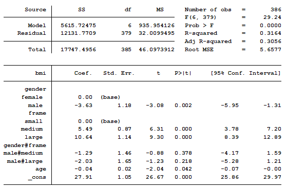
In a previous post we discussed using marginal means to explain an interaction to a non-statistical audience. The output from a linear regression model can be a bit confusing. This is the model that was shown.
In this model, BMI is the outcome variable and there are three predictors:
Age, which is continuous
Gender, which has two categories.
Frame, which has three categories.
The model also contains an interaction between the two categorical predictors. The problem with interactions between two categorical predictors is their regression coefficients are not intuitive.
The categorical interaction is measuring the difference in mean differences among specific categories. Let’s start with the coefficient for male/medium frame. Its value is -1.29. What does that actually mean?
Using the information from the table of marginal means will help us understand the difference in mean differences.
We begin by determining which category is the base index (a.k.a. reference category) for each of the two categorical variables in the interaction. Looking at the table we see that the base index for gender is female and the base index for frame is small.
(Luckily Stata actually labelled that, but if you’re using another software, the base is generally either the category that has a 0.0 value for the coefficient or is the one that is not included in the table at all).
Knowing these is important because all the coefficients measure mean differences between the labelled category and the base category.
For example, the coefficient of 5.49 tells us that the mean BMI of Medium-framed females (at the same age) is 5.49 units larger than the mean BMI of Small-Framed Females.
Table of Marginal Means
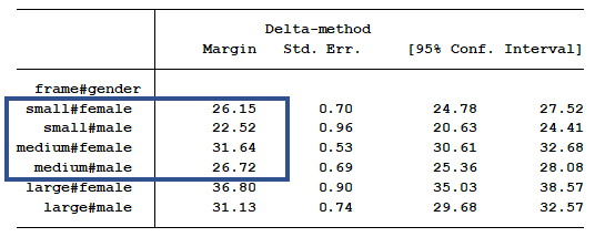
We can verify that if we just do a little subtraction looking at our marginal means table. These marginal means are already controlling for age, so we don’t have to worry about any age effects.
Indeed, the mean for Medium-framed Females (31.64) is 5.49 units larger than Small-framed Females (26.15).
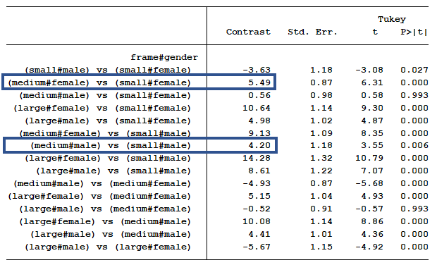
You can do this subtraction yourself or you can get your software to print out all the mean differences in another table. There will probably be more mean differences than you want, so I’ve highlighted the part we care about in blue.
Table of Differences in Marginal Means
Okay, but what about that interaction?
Remember the interaction measures the difference in the mean differences. We’ve already compared one mean difference between medium and small-framed females.
The interaction term for medium frame measures whether the mean difference between medium-framed and small-framed males is exactly the same as it was for females. Yes, it’s labelled only male#medium, but that’s why it’s important to keep your base categories in mind.
Think about this for a moment: if the difference is 0, that tells you something—the difference in mean BMI between medium and small frame is exactly the same for males and females.
The coefficient of the male#medium interaction is calculated in the following manner. First find the difference between medium frame males and small frame males. Next find the difference between medium frame females and small frame females.
Medium frame males less small frame males equal 26.72 – 22.52 =4.20.
Medium frame females less small frame females equal 31.64 – 26.15 =5.49.
Next we take the difference, 4.20 – 5.49 = -1.29. This matches the coefficient of the interaction for medium frame males.
How do we know if the difference of mean differences of 1.29 is statistically significant?
Well, that’s the beauty of the original regression coefficients table. It calculated the p-value for the null hypothesis that this difference in mean differences is 0. Where did it get that?
The statistical software package calculated a standard error of 1.46 for this parameter. We divide the coefficient by the standard error to calculate the t score. Dividing -1.29 by 1.46 is -0.88. Using a t-score table we find that a t-score of 0.88 gives us a p-value of 0.378. Thus, the interaction of gender/frame for medium frame males is not statistically significant.
So if we need a measurement and p-value for the difference in mean differences, we get that from the regression table. It tells us whether the mean BMI difference between medium and small frame males is the same as the mean BMI difference between medium and small frame females.
And in fact, our p-value of .378 indicated we have no evidence that these two mean differences are different from each other.
The pairwise comparison is a much simpler calculation. It is simply comparing the marginal means of two groups. We do not have to take the difference of the differences as we did above.
The difference between medium frame women and small frame females is 5.49. The statistical software calculated a standard error of 0.87. Dividing 5.49 by 0.87 is 6.31. The p-value of a t-score equal to 6.31 is 0.000.
So if we need a measurement and p-value for a mean differences, we get that from the table of pairwise comparisons. It tells us whether the mean BMI difference between medium and small frame males is the same as 0.
And our p-value below .0001 indicated we do have evidence that this one mean difference of 5.49 is different from 0.
That’s testing a different hypothesis than the interaction is.
Jeff Meyer is a statistical consultant with The Analysis Factor, a stats mentor for Statistically Speaking membership, and a workshop instructor. Read more about Jeff here.

It’s typically advised to adjust for multiple comparisons. Such pairwise analysis is like that. From the other side – it’s also said, that in exploratory research we rather treat p-values not in a binary “confirmatory measure”, but just “some continuous measure quantifying the discrepancy between the data and the null hypothesis”, purely “descriptively”. And the investigation of interaction seems to be such a “exploration task”. What’s your advice on that”? For example, in R we have powerful tools, like the emmeans package (for calculating LS-Means), which provides us with powerful adjustment based on multivariate t distribution, so we don’t need to use the conservative Bonferroni. But what’s the common advice? Just to run pairwise comparisons unadjusted and see what happens, as a further “hypothesis generator” (thus – informal), or adjust them all and be on the “safer side”?
This is a really hard question because there really is no good answer. There are statisticians who come down squarely on the adjust vs. don’t adjust always side. I’m not like that. I do think there are situations where you clearly always should and some where you shouldn’t, but so much depends on, for example, the relative cost of Type I vs. Type II error in that particular situation. So the best advice I can give is to consider all the issues and then explain your reasoning.
Thanks for this Jeff. What is the stata command to generate the table of difference in marginal means?
Hi Rob,
The code for producing this output was:
pwcompare frame#gender, mcomp(tukey) pveffects cformat (%6.2fc)
Jeff
Hi Jeff, In the opening paragraph you mentioned that your previous post discussed using marginal means. Could you please post the link here?
Thanks
Meenu
Hi Meenu,
You can find the previous article at this link,
https://www.theanalysisfactor.com/newsletter/December-2017.html
Thanks Jeff. Both these elaborated posts are extremely helpful. I just have a followup question:
From regression table, Am i correct to say that” With one year increase in AGE, the mean BMI of small-framed females decreases by 0.04 unit”
I feel something is incomplete in this sentence. I am just trying to interpret age when other variables and interactions are in the model.
Thanks so much
meenu
In the model shown above, there is no interaction between age and either of the other two factors (gender and frame). As a result, all six of the sub-groups (for example, small frame females) share the same slope of age. For every one year increase in age, BMI decreases by 0.04 units, regardless of body frame or gender.
We would have to use a three way interaction between gender, frame and age to find out if each sub-group has a different slope for age.
Jeff