A Note from Karen
 It's official: Our membership program, previously known as Data Analysis Brown Bag, is now called Statistically Speaking (cue applause). It's official: Our membership program, previously known as Data Analysis Brown Bag, is now called Statistically Speaking (cue applause).
We find this name better reflects the wide range of statistical support and community the program entails.
The big reveal has been underway for the past month, so you already may have noticed some changes at our website. We hope you like the new name as much as we do.
In response to customer requests, we also just rolled out a new group membership discount. So if you've been waiting for the perfect moment to join, this just might be it. Grab two or more of your closest friends or work buddies to take advantage of our 15% discount on our already affordable memberships. (Head over here for more details.)
This month we bring you an article on removing the constant from a regression model, courtesy of Jeff Meyer. And if this article piques your interest or if you've been thinking of learning Stata, be sure to check out Jeff's upcoming workshop, Introduction to Data Analysis with Stata. Enrollment closes September 29th.
Happy analyzing!
Karen
The Impact of Removing the Constant from a Regression Model: The Categorical Case
 by Jeff Meyer, MPA, MBA by Jeff Meyer, MPA, MBA
In a simple linear regression model how the constant (aka, intercept) is interpreted depends upon the type of predictor (independent) variable.
If the predictor is categorical and dummy-coded, the constant is the mean value of the outcome variable for the reference category only. If the predictor variable is continuous, the constant equals the predicted value of the outcome variable when the predictor variable equals zero.
Removing the Constant When the Predictor Is Categorical
When your predictor variable X is categorical, the results are logical. Let's look at an example.
I regressed the weight of an auto on where the auto was manufactured (domestic vs foreign) to produce the following results.
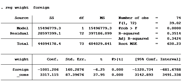
Look at the Coef. column. It tells us the mean weight of a car built domestically is 3,317 pounds. A car built outside of the U.S. weighs 1,001 pounds less, on average 2,316 pounds.
Most statistical software packages give you the option of removing the constant. This can save you the time of doing the math to determine the average weight of foreign built cars.
The model below includes the option of removing the constant.
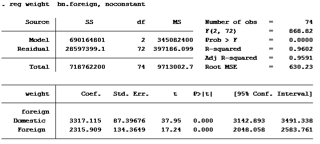
The domestic weight is the same in both outputs. In the output without the constant the mean weight of a foreign built car is shown rather than the difference in weight between domestic and foreign built cars.
Notice that the sum of the square errors (Residuals) is identical in both outputs (2,8597,399). The t-score for domestically built cars is identical in both models. The t-score for foreign is different in each model because it is measuring different statistics.
The Impact on R-squared
The one statistical measurement that is very different between the two models is the R-squared. When including the constant the R-squared is 0.3514 and when excluding the constant it is 0.9602. Wow, makes you want to run every linear regression without the constant!
The formula used for calculating R-squared without the constant is incorrect. The reported value can actually vary from one statistical software package to another. (This article explains the error in the formula, in case you're interested.)
If you are using Stata and you want the output to be similar to the “no constant” model and want accurate R-squared values then you need to use the option hascons rather than noconstant.
The impact of removing the constant when the predictor variable is continuous is significantly different. In a follow-up article, we will explore why you should never do that.
References and Further Reading:
|