If you’ve ever worked with multilevel models, you know that they are an extension of linear models. For a researcher learning them, this is both good and bad news.
The good side is that many of the concepts, calculations, and results are familiar. The down side of the extension is that everything is more complicated in multilevel models.
This includes power and sample size calculations. (more…)
If you’ve ever done any sort of repeated measures analysis or mixed models, you’ve probably heard of the unstructured covariance matrix. They can be extremely useful, but they can also blow up a model if not used appropriately. In this article I will investigate some situations when they work well and some when they don’t work at all.
The Unstructured Covariance Matrix
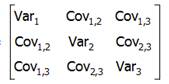 The easiest to understand, but most complex to estimate, type of covariance matrix is called an unstructured matrix. Unstructured means you’re not imposing any constraints on the values. For example, if we had a good theoretical justification that all variances were equal, we could impose that constraint and have to only estimate one variance value for every variance in the table.
But in an unstructured covariance matrix there are no constraints. Each (more…)
If you learned much about calculating power or sample sizes in your statistics classes, chances are, it was on something very, very simple, like a z-test.
But there are many design issues that affect power in a study that go way beyond a z-test. Like:
- repeated measures
- clustering of individuals
- blocking
- including covariates in a model
Regular sample size software can accommodate some of these issues, but not all. And there is just something wonderful about finding a tool that does just what you need it to.
Especially when it’s free.
Enter Optimal Design Plus Empirical Evidence software. (more…)
Generalized linear models, linear mixed models, generalized linear mixed models, marginal models, GEE models. You’ve probably heard of more than one of them and you’ve probably also heard that each one is an extension of our old friend, the general linear model.
This is true, and they extend our old friend in different ways, particularly in regard to the measurement level of the dependent variable and the independence of the measurements. So while the names are similar (and confusing), the distinctions are important.
It’s important to note here that I am glossing over many, many details in order to give you a basic overview of some important distinctions. These are complicated models, but I hope this overview gives you a starting place from which to explore more. (more…)
“Because mixed models are more complex and more flexible than the general linear model, the potential for confusion and errors is higher.”
– Hamer & Simpson (2005)
Linear Mixed Models, as implemented in SAS’s Proc Mixed, SPSS Mixed, R’s LMER, and Stata’s xtmixed, are an extension of the general linear model. They use more sophisticated techniques for estimation of parameters (means, variances, regression coefficients, and standard errors), and as the quotation says, are much more flexible.
Here’s one example of the flexibility of mixed models, and its resulting potential for confusion and error. (more…)
“Everything should be made as simple as possible, but no simpler” – Albert Einstein*
For some reason, I’ve heard this quotation 3 times in the past 3 days. Maybe I hear it everyday, but only noticed because I’ve been working with a few clients on model selection, and deciding how much to simplify a model.
And when the quotation fits, use it. (That’s the saying, right?)
*For the record, a quick web search indicated this may be a paraphrase, but it still applies.
The quotation is the general goal of model selection. You really do want the model to be as simple as possible, but still able to answer the research question of interest.
This applies to many areas of model selection. Here are a few examples: (more…)