What is the difference between Clustered, Longitudinal, and Repeated Measures Data? You can use mixed models to analyze all of them. But the issues involved and some of the specifications you choose will differ.
Just recently, I came across a nice discussion about these differences in West, Welch, and Galecki’s (2007) excellent book, Linear Mixed Models.
It’s a common question. There is a lot of overlap in both the study design and in how you analyze the data from these designs.
West et al give a very nice summary of the three types. Here’s a paraphrasing of the differences as they explain them:
- In clustered data, the dependent variable is measured once for each subject, but the subjects themselves are somehow grouped (student grouped into classes, for example). There is no ordering to the subjects within the group, so their responses should be equally correlated.
- In repeated measures data, the dependent variable is measured more than once for each subject. Usually, there is some independent variable (often called a within-subject factor) that changes with each measurement.
- In longitudinal data, the dependent variable is measured at several time points for each subject, often over a relatively long period of time.
A Few Observations
West and colleagues also make the following good observations:
1. Dropout is usually not a problem in repeated measures studies, in which all data collection occurs in one sitting. It is a huge issue in longitudinal studies, which usually require multiple contacts with participants for data collection.
2. Longitudinal data can also be clustered. If you follow those students for two years, you have both clustered and longitudinal data. You have to deal with both.
3. It can be hard to distinguish between repeated measures and longitudinal data if the repeated measures occur over time. [My two cents: A pre/post/followup design is a classic example].
4. From an analysis point of view, it doesn’t really matter which one you have. All three are types of hierarchical, nested, or multilevel data. You would analyze them all with some sort of mixed or multilevel analysis. You may of course have extra issues (like dropout) to deal with in some of these.
My Own Observations
I agree with their observations, and I’d like to add a few from my own experience.
1. Repeated measures don’t have to be repeated over time. They can be repeated over space (the right knee gets the control operation and the left knee gets the experimental operation). They can also be repeated over condition (each subject gets both the high and low cognitive load condition. Longitudinal studies are pretty much always over time.
This becomes an issue mainly when you are choosing a covariance structure for the within-subject residuals (as determined by the Repeated statement in SAS’s Proc Mixed or SPSS Mixed). An auto-regressive structure is often needed when some repeated measurements are closer to each other than others (over either time or space). This is not an issue with purely clustered data, since there is no order to the observations within a cluster.
2. Time itself is often an important independent variable in longitudinal studies, but in repeated measures studies, it is usually confounded with some independent variable.
When you’re deciding on an analysis, it’s important to think about the role of time. Time is not important in an experiment, where each measurement is a different condition (with order often randomized). But it’s very important in a study designed to measure changes in a dependent variable over the course of 3 decades.
3. Time may be measured with some proxy like Age or Order. But it’s still really about time.
4. A longitudinal study does not have to be over years. You could be measuring reaction time every second for a minute. In cases like this, dropout isn’t an issue, although time is an important predictor.
5. Consider whether it makes sense to think about time as continuous or categorical. If you have only two time points, even if you have numerical measurements for them, there is no point in treating it as continuous. You need at least three time points to fit a line, but more is always better.
6. Longitudinal data can be analyzed with many statistical methods, including structural equation modeling and survival analysis. You only use multilevel modeling if the dependent variable is measured repeatedly and if the point of the model is to see how it changes (or differs).
Naming a data structure, design, or analysis is most helpful if it is so specific that it defines yours exactly. Your repeated measures analysis may not be like the repeated measures example you’re trying to follow. Rather than trying to name the analysis or the data structure, think about the issues involved in your design, your hypotheses, and your data. Work with them accordingly.
Go to the next article or see the full series on Easy-to-Confuse Statistical Concepts
 If you have a categorical predictor variable that you plan to use in a regression analysis in SPSS, there are a couple ways to do it.
You can use the SPSS Regression procedure. Or you can use SPSS General Linear Model–>Univariate, which I discuss here. If you use Syntax, it’s the UNIANOVA command.
The big question in SPSS GLM is what goes where. As I’ve detailed in another post, any continuous independent variable goes into covariates. And don’t use random factors at all unless you really know what you’re doing.
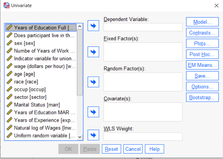
So the question is what to do with your categorical variables. You have two choices, and each has advantages and disadvantages.
The easiest is to put categorical variables in Fixed Factors. SPSS GLM will dummy code those variables for you, which is quite convenient if your categorical variable has more than two categories.
However, there are some defaults you need to be aware of that may or may not make this a good choice.
The dummy coding reference group default
SPSS GLM always makes the reference group the one that comes last alphabetically.
So if the values you input are strings, it will be the one that comes last. If those values are numbers, it will be the highest one.
Not all procedures in SPSS use this default so double check the default if you’re using something else. Some procedures in SPSS let you change the default, but GLM doesn’t.
In some studies it really doesn’t matter which is the reference group.
But in others, interpreting regression coefficients will be a whole lot easier if you choose a group that makes a good comparison such as a control group or the most common group in the data.
If you want that to be the reference group in SPSS GLM, make it come last alphabetically. I’ve been known to do things like change my data so that the control group becomes something like ZControl. (But create a new variable–never overwrite original data).
It really can get confusing, though, if the variable was already dummy coded–if it already had values of 0 and 1. Because 1 comes last alphabetically, SPSS GLM will make that group the reference group and internally code it as 0.
This can really lead to confusion when interpreting coefficients. It’s not impossible if you’re paying attention, but you do have to pay attention. It’s generally better to recode the variable so that you don’t confuse yourself. And while you may believe you’re up for overcoming the confusion, why make things harder on yourself or with any other colleague you’re sharing results with?
Interactions among fixed factors default
There is another key default to keep in mind. GLM will automatically create interactions between any and all variables you specify as Fixed Factors.
If you put 5 variables in Fixed Factors, you’ll get a lot of interactions. SPSS will automatically create all 2-way, 3-way, 4-way, and even a 5-way interaction among those 5 variables.
That’s a lot of interactions.
In contrast, GLM doesn’t create by default any interactions between Covariates or between Covariates and Fixed Factors.
So you may find you have more interactions than you wanted among your categorical predictors. And fewer interactions than you wanted among numerical predictors.
There is no reason to use the default. You can override it quite easily.
Just click on the Model button. Then choose “Custom Model.” You can then choose which interactions you do, or don’t, want in the model.
If you’re using SPSS syntax, simply add the interactions you want to the /Design subcommand.
So think about which interactions you want in the model. And take a look at whether your variables are already dummy coded.
Interpreting the Intercept in a regression model isn’t always as straightforward as it looks.
Here’s the definition: the intercept (often labeled the constant) is the expected value of Y when all X=0. But that definition isn’t always helpful. So what does it really mean?
Regression with One Predictor X
Start with a very simple regression equation, with one predictor, X.
If X sometimes equals 0, the intercept is simply the expected value of Y at that value. In other words, it’s the mean of Y at one value of X. That’s meaningful.
If X never equals 0, then the intercept has no intrinsic meaning. You literally can’t interpret it. That’s actually fine, though. You still need that intercept to give you unbiased estimates of the slope and to calculate accurate predicted values. So while the intercept has a purpose, it’s not meaningful.
Both these scenarios are common in real data. (more…)
Have you ever had this happen? You run a regression model. It can be any kind—linear, logistic, multilevel, etc. In the ANOVA table, the effect of interest has a very low p-value. In the regression table, it doesn’t. Or vice-versa.
How can the same effect have two different p-values? In this article, let’s explore when this happens and what it means.
What the statistics in each table measures
The ANOVA table is a table of F tests. It may not be called the ANOVA table on your output, but it always includes a set of F tests. Some software procedures only give one F test for the model as a whole, but most will break it down into a series of F tests, one for each predictor variable or term in your model.
The regression coefficients table is a table of t tests. It includes each regression coefficient, along with its standard error, and usually a t test (some generalized linear models will have Wald or z tests instead, but they have the same role here).
Both tables often list out each predictor variable, along with a p-value for that variable’s conditional effect on Y.
There are two situations in which the p-values will match. Both must be true.
- The F test has one df. This happens in two situations. Either the predictor, X, is numerical or it’s categorical and binary (only two groups).
- The predictor is not involved with any interactions with a variable that is not centered at is mean.
If both of those are true, not only will the p-value match, but the t-statistic in the regression coefficients table will be the positive or negative square root of the F statistic.
An Example ANOVA Table with Matching and Unmatching Regression Coefficients
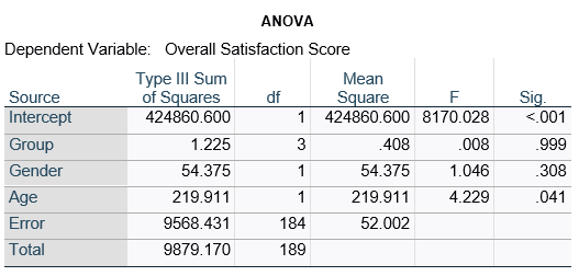
Here’s an example of an ANOVA table from a linear regression. In this example, there are four treatment groups, two genders, and age in years (measured continuously and centered at its mean). The response variable, Y, is a satisfaction score with a training. The four groups represented four learning strategies the adult learners were trained to use.
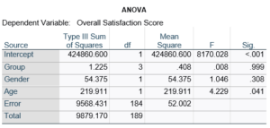
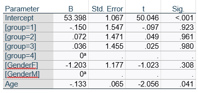
Let’s compare this to the regression coefficients table.

If you compare p-values across the two tables, you can see that Gender and Age have the same p-values, but Group doesn’t.
Gender and Age meet both conditions. Both have 1 df in the F table. Gender because it’s binary (two categories) and Age because it’s numerical). There are no interactions.
Group doesn’t match because it has 3 df in the F test. The F test is testing the null hypothesis that there is no difference among the four means. The t-tests in the regression coefficients table are testing three specific contrasts. Each one compares one group mean to the group 4 mean. For example, the group=1 coefficient tests whether the difference between the mean group 1 satisfaction score differs only from the group 4 score. It’s a different null hypothesis than the F test.
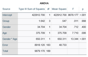
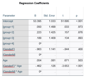
This would be the case whether or not there were interactions in the model that contain Group. Any time you have more that one df in the F test (you can see group has 3), you’ll get as many p-values in the regression coefficients as you have df in the F table. The p-values can’t match because there are more of them in the regression coefficients table.
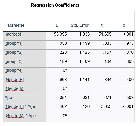
Gender, which is also categorical, does have the same p-value in both tables. It has 1 df in the F test, which tests the null hypothesis that the two gender means have no variance (they’re the same). Gender is involved in an interaction, so the only reason the hypothesis test, and therefore the p-value, is the same is because the variable it interacts with, Age, is centered.
In conclusion, most of the time, it’s fine if the results don’t match. It’s because the two tables are reporting results of different hypothesis tests, based on what’s in your model.
One of the important issues with missing data is the missing data mechanism. You may have heard of these: Missing Completely at Random (MCAR), Missing at Random (MAR), and Missing Not at Random (MNAR).
The mechanism is important because it affects how much the missing data bias your results. This has a big impact on what is a reasonable approach to dealing with the missing data. So you have to take it into account in choosing an approach.
The concepts of these mechanisms can be a bit abstract.
And to top it off, two of these mechanisms have really confusing names: Missing Completely at Random and Missing at Random.
Missing Completely at Random (MCAR)
Missing Completely at Random is pretty straightforward. What it means is what is (more…)
Some repeated measures designs make it quite challenging to specify within-subjects factors. Especially difficult is when the design contains two “levels” of repeat, but your interest is in testing just one.
Let’s look at a great example of what this looks like and how to deal with it in this question from a reader :
The Design:
I want to do a GLM (repeated measures ANOVA) with the valence of some actions of my test-subjects (valence = desirability of actions) as a within-subject factor. My subjects have to rate a number of actions/behaviours in a pre-set list of 20 actions from ‘very likely to do’ to ‘will never do this’ on a scale from 1 to 7, and some of these actions are desirable (e.g. help a blind man crossing the street) and therefore have a positive valence (in psychology) and some others are non-desirable (e.g. play loud music at night) and therefore have negative valence in psychology.
My question is how I can use valence as a within-subjects factor in GLM. Is there a way to tell SPSS some actions have positive valence and others have negative valence ? I assume assigning labels to the actions will not do it, as SPSS does not make analyses based on labels …
Please help. Thank you.
(more…)