Regression models

Time to event analyses (aka, Survival Analysis and Event History Analysis) are used often within medical, sales and epidemiological research. Some examples of time-to-event analysis are measuring the median time to death after being diagnosed with a heart condition, comparing male and female time to purchase after being given a coupon and estimating time to infection after exposure to a disease.

Survival time has two components that must be clearly defined: a beginning point and an endpoint that is reached either when the event occurs or when the follow-up time has ended.

One basic concept needed to understand time-to-event (TTE) analysis is censoring.

In simple TTE, you should have two types of observations:

1. The event occurred, and we are able to measure when it occurred OR

2. The event did NOT occur during the time we observed the individual, and we only know the total number of days in which it didn’t occur. (CENSORED).

Again you have two groups, one where the time-to-event is known exactly and one where it is not. The latter group is only known to have a certain amount of time where the event of interest did not occur. We don’t know if it would have occurred had we observed the individual longer. But knowing that it didn’t occur for so long tells us something about the risk of the envent for that person.

For example, let the time-to-event be a person’s age at onset of cancer. If you stop following someone after age 65, you may know that the person did NOT have cancer at age 65, but you do not have any information after that age.

You know that their age of getting cancer is greater than 65. But you do not know if they will never get cancer or if they’ll get it at age 66, only that they have a “survival” time greater than 65 years. They are censored because we did not gather information on that subject after age 65.

So one cause of censoring is merely that we can’t follow people forever.  At some point you have to end your study, and not all people will have experienced the event.

But another common cause is that people are lost to follow-up during a study. This is called random censoring. It occurs when follow-up ends for reasons that are not under control of the investigator.

In survival analysis, censored observations contribute to the total number at risk up to the time that they ceased to be followed.  One advantage here is that the length of time that an individual is followed does not have to be equal for everyone. All observations could have different amounts of follow-up time, and the analysis can take that into account.

Allison, P. D. (1995). Survival Analysis Using SAS. Cary, NC: SAS Institute Inc.

Hosmer, D. W. (2008). Applied Survival Analysis (2nd ed.). Hoboken, NJ: John Wiley & Sons, Inc.

1 comment

If you’re like most researchers, your statistical training focused on Regression or ANOVA, but not both. It all depends on whether your field focuses more on experimental data (Biology, Psychology) or observed data (Sociology, Economics). Maybe one class covered a bit of the other, but most people are comfortable in one, but not the other.

This, in my opinion, is a shame. (Okay, I was going to say tragedy, but let’s be real.  Tsunami that kills thousands=tragedy.  Different scale here).

First of all, the distinction between ANOVA and linear regression is arbitrary. They’re really the same model with different outfits on.

Second, regardless of which one you normally use, you’re going to occasionally have to use the other kind of predictor variables–categorical or continuous. And we can come up with nice names for these models–a regression with dummy variables or an Analysis of Covariance.

But real understanding of the relationships among variables comes only when you dispense of the names and can focus on analyzing and interpreting the model using the kinds of variables you have.

There are other examples, but today I’m going to focus on an ANOVA model with a continuous covariate.

A common model is one in which one predictor is categorical (we’ll use 4 categories) and the other is continuous. Here is an example of a scatterplot of just such a model:

There are four groups, each of which received a different training.  The continuous moderator is Age, and the outcome is OverallPost, which is the post-training test score to see how well they learned the material in each training program.

As you can see, the effect of the training program is moderated by age.  Another way to say that is there is a significant interaction between Age and Training Group.  The effect of the training is depending on the trainee’s age.

One way to interpret this significant interaction is to compare the slopes of the four lines, which is easily done with any regression coefficient table.  (Okay, not always easily done, but easily found in…)

But this doesn’t make very much sense when Age is really a moderator–a predictor we want to control for, and see how it affects the relationship between the independent (IV) and dependent variables (DV), but not really the IV we’re interested in.

A better way to do it in this situation is to compare the means among groups at a low value of Age, say 20, and again at a high value of Age, say 50.  You can get p-values, adjusted for multiple comparisons, using either SAS or SPSS GLM.

SAS Proc GLM uses the LSMeans statement and SPSS GLM uses EMMeans.  They do the same thing–calculate the mean of Y for each group, at a specific value of the covariate.

If you use the menus in SPSS, you can only get those EMMeans at the Covariate’s mean, which in this example is about 25, where the vertical black line is.  This isn’t very useful for our purposes.  But we can change the value of the covariate at which to compare the means using syntax.

So it would tell us that at a young age of say 20, the three treatment groups (green, tan, and purple lines) all have means higher than the control (blue).  Young people learned more in all three treatment groups.

But at an older age, say 50, the means of the purple and tan groups were not significantly different from the control group’s (blue), and the green  (EIQ group) did worse!

In SPSS GLM, the syntax would be:

UNIANOVA OverallPost BY group WITH NEWAGE
/METHOD=SSTYPE(3)
/INTERCEPT=INCLUDE
/EMMEANS=TABLES(group) WITH(NEWAGE=MEAN) COMPARE ADJ(SIDAK)
/EMMEANS=TABLES(group) WITH(NEWAGE=45) COMPARE ADJ(SIDAK)
/EMMEANS=TABLES(group) WITH(NEWAGE=20) COMPARE ADJ(SIDAK)
/PRINT=PARAMETER
/CRITERIA=ALPHA(.05)
/DESIGN=NEWAGE group NEWAGE*group.

 

1 comment

Just recently, a client got some feedback from a committee member that the Analysis of Covariance (ANCOVA) model she ran did not meet all the assumptions.

Specifically, the assumption in question is that the covariate has to be uncorrelated with the independent variable.

This committee member is, in the strictest sense of how analysis of covariance is used, correct.

And yet, they over-applied that assumption to an inappropriate situation.

ANCOVA for Experimental Data

Analysis of Covariance was developed for experimental situations and some of the assumptions and definitions of ANCOVA apply only to those experimental situations.

The key situation is the independent variables are categorical and manipulated, not observed.

The covariate–continuous and observed–is considered a nuisance variable. There are no research questions about how this covariate itself affects or relates to the dependent variable.

The only hypothesis tests of interest are about the independent variables, controlling for the effects of the nuisance covariate.

A typical example is a study to compare the math scores of students who were enrolled in three different learning programs at the end of the school year.

The key independent variable here is the learning program. Students need to be randomly assigned to one of the three programs.

The only research question is about whether the math scores differed on average among the three programs. It is useful to control for a covariate like IQ scores, but we are not really interested in the relationship between IQ and math scores.

So in this example, in order to conclude that the learning program affected math scores, it is indeed important that IQ scores, the covariate, is unrelated to which learning program the students were assigned to.

You could not make that causal interpretation if it turns out that the IQ scores were generally higher in one learning program than the others.

So this assumption of ANCOVA is very important in this specific type of study in which we are trying to make a specific type of inference.

ANCOVA for Other Data

But that’s really just one application of a linear model with one categorical and one continuous predictor. The research question of interest doesn’t have to be about the causal effect of the categorical predictor, and the covariate doesn’t have to be a nuisance variable.

A regression model with one continuous and one dummy-coded variable is the same model (actually, you’d need two dummy variables to cover the three categories, but that’s another story).

The focus of that model may differ–perhaps the main research question is about the continuous predictor.

But it’s the same mathematical model.

The software will run it the same way. YOU may focus on different parts of the output or select different options, but it’s the same model.

And that’s where the model names can get in the way of understanding the relationships among your variables. The model itself doesn’t care if the categorical variable was manipulated. It doesn’t care if the categorical independent variable and the continuous covariate are mildly correlated.

If those ANCOVA assumptions aren’t met, it does not change the analysis at all. It only affects how parameter estimates are interpreted and the kinds of conclusions you can draw.

In fact, those assumptions really aren’t about the model. They’re about the design. It’s the design that affects the conclusions. It doesn’t matter if a covariate is a nuisance variable or an interesting phenomenon to the model. That’s a design issue.

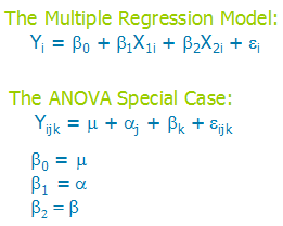
The General Linear Model

So what do you do instead of labeling models? Just call them a General Linear Model. It’s hard to think of regression and ANOVA as the same model because the equations look so different. But it turns out they aren’t.

If you look at the two models, first you may notice some similarities.

• Both are modeling Y, an outcome.
• Both have a “fixed” portion on the right with some parameters to estimate–this portion estimates the mean values of Y at the different values of X.
• Both equations have a residual, which is the random part of the model. It is the variation in Y that is not affected by the Xs.

But wait a minute, Karen, are you nuts?–there are no Xs in the ANOVA model!

Actually, there are. They’re just implicit.

Since the Xs are categorical, they have only a few values, to indicate which category a case is in. Those j and k subscripts? They’re really just indicating the values of X.

(And for the record, I think a couple Xs are a lot easier to keep track of than all those subscripts.  Ever have to calculate an ANOVA model by hand?  Just sayin’.)

So instead of trying to come up with the right label for a model, focus instead on understanding (and describing in your paper) the measurement scales of your variables, if and how much they’re related, and how that affects the conclusions.

In my client’s situation, it was not a problem that the continuous and the categorical variables were mildly correlated. The data were not experimental and she was not trying to draw causal conclusions about only the categorical predictor.

So she had to call this ANCOVA model a multiple regression.

18 comments

Whenever I get email questions whose answers I think would benefit others, I like to answer them here.  I leave out the asker’s name for privacy, but this is a great question about dummy coding:

First of all, thanks for all those helpful information you provided! Thanks sincerely for all your efforts!

Actually I am here to ask a technical question. See, I have 6 locations (let’s say A, B, C, D, E, and F), and I want to see the location effect on the outcome using OLS models.

I know that if I included 5 dummy location variables (6 locations in total, with A as the reference group) in 1 block of the regression analysis, the result would be based on the comparison with the reference location.

Then what if I put 6 dummies (for example, the 1st dummy would be “1” for A location, and “0” for otherwise) in 1 block? Will it be a bug? If not, how to interpret the result?

Thanks a lot!

Great question!

If you put in a 6th dummy code for Location A, your reference group, the model will actually blow up. (Yes, that’s a technical term).

This is one of those cases of pure multicollinearity, and the model can’t be estimated uniquely.

It’s the same situation you learned back in Algebra where you have two equations, one unknown.  The problem isn’t that it can’t be solved–the problem is there are an infinite number of equally good solutions.

If an observation falls in Location A, the reference group, we’ve already gotten that information from the other 5 dummy variables.  That observation would have a 0 on all of them.  So we already know it’s location is A.  We don’t need another dummy variable to tell the model that.  It’s redundant information.  And so perfectly redundant that the model will choke.

Dummy coding is one of the topics I get the most questions about.  It can get especially tricky to interpret when the dummy variables are also used in interactions, so I’ve created some resources that really dig in deeply.

1 comment

In a previous post, Interpreting Interactions in Regression, I said the following:

In our example, once we add the interaction term, our model looks like:

Height = 35 + 4.2*Bacteria + 9*Sun + 3.2*Bacteria*Sun

Adding the interaction term changed the values of B1 and B2. The effect of Bacteria on Height is now 4.2 + 3.2*Sun. For plants in partial sun, Sun = 0, so the effect of Bacteria is 4.2 + 3.2*0 = 4.2. So for two plants in partial sun, a plant with 1000 more bacteria/ml in the soil would be expected to be 4.2 cm taller than a (more…)

8 comments

There are many types of outcome variables that don’t work in linear models, but look like they should. (I mean, specifically, OLS regression and ANOVA models).

They include discrete counts; truncated or censored variables, where part of the distribution is cut off or measured only up to a certain point; and bounded variables, like proportions and percentages.

This article outlines a particular type of outcome variable: one that measures whether or when an event occurs. They are typically called (more…)

No comments yet