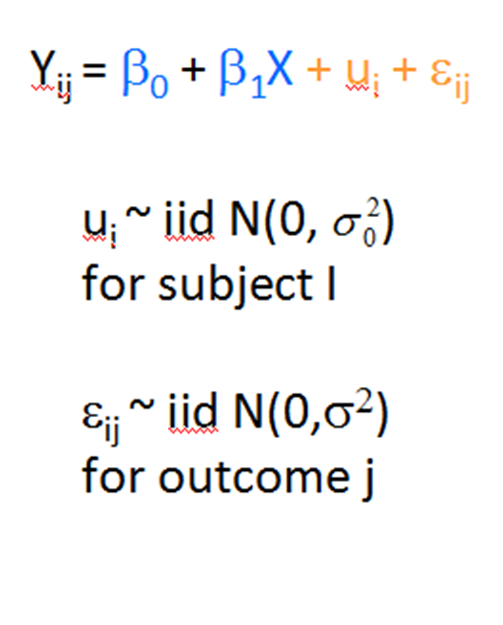
• Skip to primary navigation
  • Skip to main content
  • Skip to primary sidebar
The Analysis Factor

The Analysis Factor

Statistical Consulting, Resources, and Statistics Workshops for Researchers

  • our programs
    • Membership
    • Online Workshops
    • Free Webinars
    • Consulting Services
  • statistical resources
  • blog
  • about
    • Our Team
    • Our Core Values
    • Our Privacy Policy
    • Employment
    • Collaborate with Us
  • contact
  • login

Karen Grace-Martin

Can Likert Scale Data ever be Continuous?

by Karen Grace-Martin  51 Comments

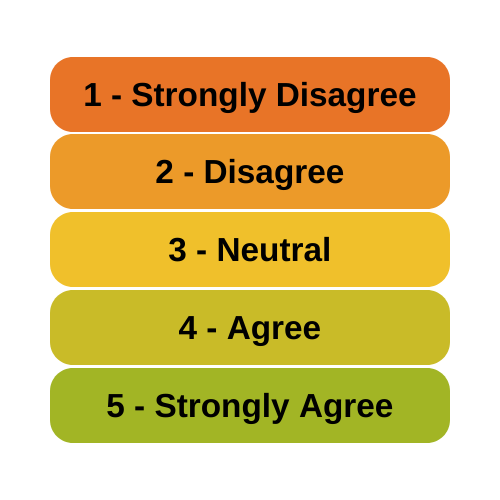
A very common question is whether it is legitimate to use Likert scale data in parametric statistical procedures that 
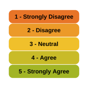
require interval data, such as Linear Regression, ANOVA, and Factor Analysis.

A typical Likert scale item has 5 to 11 points that indicate the degree of something. For example, it could measure agreement with a statement, such as 1=Strongly Disagree to 5=Strongly Agree. It can be a 1 to 5 scale, 0 to 10, etc. [Read more…] about Can Likert Scale Data ever be Continuous?

Tagged With: ANOVA, continuous variable, Factor Analysis, Likert Scale, linear regression, Model Assumptions, Nonparametric statistics

Related Posts

  • Beyond Median Splits: Meaningful Cut Points
  • Checking Assumptions in ANOVA and Linear Regression Models: The Distribution of Dependent Variables
  • Member Training: The Link Between ANOVA and Regression
  • Member Training: Centering

Getting Started with SPSS Syntax

by Karen Grace-Martin  Leave a Comment

spss-logoYou may have heard that using SPSS syntax is more efficient, gives you more control, and ultimately saves you time and frustration.  It’s all true.

….And yet you probably use SPSS because you don’t want to code.  You like the menus.

I get it.

I like the menus, too, and I use them all the time.

But I use syntax just as often.

At some point, if you want to do serious data analysis, you have to start using syntax.  [Read more…] about Getting Started with SPSS Syntax

Tagged With: SPSS, spss syntax, Statistical Software

Related Posts

  • Member Training: Introduction to SPSS Software Tutorial
  • How to do a Chi-square test when you only have proportions and denominators
  • SPSS, SAS, R, Stata, JMP? Choosing a Statistical Software Package or Two
  • Averaging and Adding Variables with Missing Data in SPSS

Three SPSS Shortcuts that Make Life Easier

by Karen Grace-Martin  1 Comment

Okay, maybe these SPSS shortcuts won’t make your whole life easier, but it will help your work life, at least the SPSS part of it.

When I consult with researchers, a common part of that is going through their analysis together.  Sometimes I notice that they’re using some shortcut in SPSS that I had not known about.

Or sometimes they could be saving themselves some headaches.

So I thought I’d share three buttons you may not have noticed before that will make your data analysis more efficient.

[Read more…] about Three SPSS Shortcuts that Make Life Easier

Tagged With: spss shortcuts

Related Posts

  • Getting Started with SPSS Syntax
  • How to do a Chi-square test when you only have proportions and denominators
  • Member Training: Introduction to SPSS Software Tutorial
  • Tricks for Using Word to Make Statistical Syntax Easier

Specifying Fixed and Random Factors in Mixed Models

by Karen Grace-Martin  13 Comments

One of the difficult decisions in mixed modeling is deciding which factors are fixed and which are random. And as difficult as it is, it’s also very important. Correctly specifying the fixed and random factors of the model is vital to obtain accurate analyses.

Now, you may be thinking of the fixed and random effects in the model, rather than the factors themselves, as fixed or random. If so, remember that each term in the model (factor, covariate, interaction or other multiplicative term) has an effect. We’ll come back to how the model measures the effects for fixed and random factors.

Sadly, the definitions in many texts don’t help much with decisions to specify factors as fixed or random. Textbook examples are often artificial and hard to apply to the real, messy data you’re working with.

Here’s the real kicker. The same factor can often be fixed or random, depending on the researcher’s objective.

That’s right, there isn’t always a right or a wrong decision here. It depends on the inferences you want to make about this factor. This article outlines a different way to think about fixed and random factors.

An Example

Consider an experiment that examines beetle damage on cucumbers. The researcher replicates the experiment at five farms and on four fields at each farm.

There are two varieties of cucumbers, and the researcher measures beetle damage on each of 50 plants at the end of the season. The researcher wants to measure differences in how much damage the two varieties sustain.

The experiment then has the following factors: VARIETY, FARM, and FIELD.

Fixed factors can be thought of in terms of differences.

The effect of a categorical fixed factor is measured by differences from the overall mean.

The effect of a continuous fixed predictor (usually called a covariate) is defined by its slope–how the mean of the dependent variable differs with differing values of the predictor.

The output for fixed predictors, then, gives estimates for mean-differences or slopes.

Conclusions regarding fixed factors are particular to the values of these factors. For example, if one variety of cucumber has significantly less damage than the other, you can make conclusions about these two varieties. This says nothing about cucumber varieties that were not tested.

Random factors, on the other hand, are defined by a distribution and not by differences.

The values of a random factor are assumed to be chosen from a population with a normal distribution with a certain variance.

The output for a random factor is an estimate of this variance and not a set of differences from a mean. Effects of random factors are measured in terms of variance, not mean differences.

For example, we may find that the variance among fields makes up a certain percentage of the overall variance in beetle damage. But we’re not measuring how much higher the beetle damage is in one field compared to another. We only care that they vary, not how much they differ.

Software specification of fixed and random factors

Before we get into specifying factors as fixed and random, please note:

When you’re specifying random effects in software, like intercepts and slopes, the random factor is itself the Subject variable in your software. This differs in different software procedures. Some specifically ask for code like “Subject=FARM.” Others just put FARM after a || or some other indicator of the subject for which random intercepts and slopes are measured.

Some software, like SAS and SPSS, allow you to specify the random factors two ways. One is to list the random effects (like intercept) along with the random factor listed as a subject.

/Random Intercept | Subject(Farm)

The other is to list the random factors themselves.

/Random Farm

Both of those give you the same output.

Other software, like R and Stata, only allow the former. And neither uses the term “Subject” anywhere. But that random factor, the subject, still needs to be specified after the | or || in the random part of the model.

Specifying fixed effects is pretty straightforward.

Situations that indicate a factor should be specified as fixed:

1. The factor is the primary treatment that you want to compare.

In our example, VARIETY is definitely fixed as the researcher wants to compare the mean beetle damage on the two varieties.

2. The factor is a secondary control variable, and you want to control for differences in the specific values of this factor.

Say the researcher chose these farms specifically for some feature they had, such as specific soil types or topographies that may affect beetle damage. If the researcher wants to compare the farms as representatives of those soil types, then FARM should be fixed.

3. The factor has only two values.

Even if everything else indicates that a factor should be random, if it has only two values, the variance cannot be calculated, and it should be fixed.

Situations that indicate random factors:

1. Your interest is in quantifying how much of the overall variance to attribute to this factor.

If you want to know how much of the variation in beetle damage you can attribute to the farm at which the damage took place, FARM would be random.

2. Your interest is not in knowing which specific means differ, but you want to account for the variation in this factor.

If the farms were chosen at random, FARM should be random.

This choice of the specific farms involved in the study is key. If you can rerun the study using different specific farms–different values of the Farm factor–and still be able to draw the same conclusions, then Farm should be random. However, if you want to compare or control for these particular farms, then Farm is a fixed factor.

3. You would like to generalize the conclusions about this factor to the whole population.

There is nothing about comparing these specific fields that is of interest to the researcher. Rather, the researcher wants to generalize the results of this experiment to all fields, so FIELD is random.

4. Any interaction with a random factor is also random.

How the factors of a model are specified can have great influence on the results of the analysis and on the conclusions drawn.


Tagged With: Fixed Factor, mixed model, multilevel model, Proc Mixed, Random Factor, S-Plus, SAS, SPSS, Stata

Related Posts

  • Multilevel, Hierarchical, and Mixed Models–Questions about Terminology
  • The Difference Between Random Factors and Random Effects
  • Confusing Statistical Terms #3: Level
  • The Difference Between Crossed and Nested Factors

Interpreting Regression Coefficients

by Karen Grace-Martin  31 Comments

Updated 12/20/2021

Despite its popularity, interpreting regression coefficients of any but the simplest models is sometimes, well….difficult.

So let’s interpret the coefficients in a model with two predictors: a continuous and a categorical variable.  The example here is a linear regression model. But this works the same way for interpreting coefficients from any regression model without interactions.

A linear regression model with two predictor variables results in the following equation:

Yi = B0 + B1*X1i + B2*X2i + ei.

The variables in the model are:

  • Y, the response variable;
  • X1, the first predictor variable;
  • X2, the second predictor variable; and
  • e, the residual error, which is an unmeasured variable.

The parameters in the model are:

  • B0, the Y-intercept;
  • B1, the first regression coefficient; and
  • B2, the second regression coefficient.

One example would be a model of the height of a shrub (Y) based on the amount of bacteria in the soil (X1) and whether the plant is located in partial or full sun (X2).

Height is measured in cm. Bacteria is measured in thousand per ml of soil.  And type of sun = 0 if the plant is in partial sun and type of sun = 1 if the plant is in full sun.

Let’s say it turned out that the regression equation was estimated as follows:

Y = 42 + 2.3*X1 + 11*X2

Interpreting the Intercept

B0, the Y-intercept, can be interpreted as the value you would predict for Y if both X1 = 0 and X2 = 0.

We would expect an average height of 42 cm for shrubs in partial sun with no bacteria in the soil. However, this is only a meaningful interpretation if it is reasonable that both X1 and X2 can be 0, and if the data set actually included values for X1 and X2 that were near 0.

If neither of these conditions are true, then B0 really has no meaningful interpretation. It just anchors the regression line in the right place. In our case, it is easy to see that X2 sometimes is 0, but if X1, our bacteria level, never comes close to 0, then our intercept has no real interpretation.

Interpreting Coefficients of Continuous Predictor Variables

Since X1 is a continuous variable, B1 represents the difference in the predicted value of Y for each one-unit difference in X1, if X2 remains constant.

This means that if X1 differed by one unit (and X2 did not differ) Y will differ by B1 units, on average.

In our example, shrubs with a 5000/ml bacteria count would, on average, be 2.3 cm taller than those with a 4000/ml bacteria count. They likewise would be about 2.3 cm taller than those with 3000/ml bacteria, as long as they were in the same type of sun.

(Don’t forget that since the measurement unit for bacteria count is 1000 per ml of soil, 1000 bacteria represent one unit of X1).

Interpreting Coefficients of Categorical Predictor Variables

Similarly, B2 is interpreted as the difference in the predicted value in Y for each one-unit difference in X2 if X1 remains constant. However, since X2 is a categorical variable coded as 0 or 1, a one unit difference represents switching from one category to the other.

B2 is then the average difference in Y between the category for which X2 = 0 (the reference group) and the category for which X2 = 1 (the comparison group).

So compared to shrubs that were in partial sun, we would expect shrubs in full sun to be 11 cm taller, on average, at the same level of soil bacteria.

Interpreting Coefficients when Predictor Variables are Correlated

Don’t forget that each coefficient is influenced by the other variables in a regression model. Because predictor variables are nearly always associated, two or more variables may explain some of the same variation in Y.

Therefore, each coefficient does not measure the total effect on Y of its corresponding variable. It would if it were the only predictor variable in the model. Or if the predictors were independent of each other.

Rather, each coefficient represents the additional effect of adding that variable to the model, if the effects of all other variables in the model are already accounted for.

This means that adding or removing variables from the model will change the coefficients. This is not a problem, as long as you understand why and interpret accordingly.

Interpreting Other Specific Coefficients

I’ve given you the basics here. But interpretation gets a bit trickier for more complicated models, for example, when the model contains quadratic or interaction terms. There are also ways to rescale predictor variables to make interpretation easier.

So here is some more reading about interpreting specific types of coefficients for different types of models:

  • Interpreting the Intercept
  • Removing the Intercept when X is Continuous or Categorical
  • Interpreting Interactions in Regression
  • How Changing the Scale of X affects Interpreting its Regression Coefficient
  • Interpreting Coefficients with a Centered Predictor

Tagged With: categorical predictor, continuous predictor, Intercept, interpreting regression coefficients, linear regression

Related Posts

  • Centering a Covariate to Improve Interpretability
  • Using Marginal Means to Explain an Interaction to a Non-Statistical Audience
  • Member Training: Segmented Regression
  • Should You Always Center a Predictor on the Mean?

Member Training: Matrix Algebra for Data Analysts: A Primer

by Karen Grace-Martin  4 Comments

If you’ve been doing data analysis for very long, you’ve certainly come across terms, concepts, and processes of matrix algebra.  Not just matrices, but:

  • Matrix addition and multiplication
  • Traces and determinants
  • Eigenvalues and Eigenvectors
  • Inverting and transposing
  • Positive and negative definite

[Read more…] about Member Training: Matrix Algebra for Data Analysts: A Primer

Tagged With: Factor Analysis, linear, matrix, mixed model, multivariate analysis

Related Posts

  • Member Training: Goodness of Fit Statistics
  • Member Training: Generalized Linear Models
  • Member Training: Power Analysis and Sample Size Determination Using Simulation
  • Member Training: Confirmatory Factor Analysis

  • Go to page 1
  • Go to page 2
  • Go to page 3
  • Interim pages omitted …
  • Go to page 19
  • Go to Next Page »

Primary Sidebar

This Month’s Statistically Speaking Live Training

  • Member Training: Moderated Mediation, Not Mediated Moderation

Upcoming Workshops

    No Events

Upcoming Free Webinars

TBA

Quick links

Our Programs Statistical Resources Blog/News About Contact Log in

Contact

Upcoming

Free Webinars Membership Trainings Workshops

Privacy Policy

Search

Copyright © 2008–2023 The Analysis Factor, LLC.
All rights reserved.

The Analysis Factor uses cookies to ensure that we give you the best experience of our website. If you continue we assume that you consent to receive cookies on all websites from The Analysis Factor.
Continue Privacy Policy
Privacy & Cookies Policy

Privacy Overview

This website uses cookies to improve your experience while you navigate through the website. Out of these, the cookies that are categorized as necessary are stored on your browser as they are essential for the working of basic functionalities of the website. We also use third-party cookies that help us analyze and understand how you use this website. These cookies will be stored in your browser only with your consent. You also have the option to opt-out of these cookies. But opting out of some of these cookies may affect your browsing experience.
Necessary
Always Enabled
Necessary cookies are absolutely essential for the website to function properly. This category only includes cookies that ensures basic functionalities and security features of the website. These cookies do not store any personal information.
Non-necessary
Any cookies that may not be particularly necessary for the website to function and is used specifically to collect user personal data via analytics, ads, other embedded contents are termed as non-necessary cookies. It is mandatory to procure user consent prior to running these cookies on your website.
SAVE & ACCEPT