Imputation as an approach to missing data has been around for decades.

You probably learned about mean imputation in methods classes, only to be told to never do it for a variety of very good reasons. Mean imputation, in which each missing value is replaced, or imputed, with the mean of observed values of that variable, is not the only type of imputation, however. (more…)

Missing data causes a lot of problems in data analysis. Unfortunately, some of the “solutions” for missing data cause more problems than they solve.
(more…)
Mean imputation: So simple. And yet, so dangerous.
Perhaps that’s a bit dramatic, but mean imputation (also called mean substitution) really ought to be a last resort.
It’s a popular solution to missing data, despite its drawbacks. Mainly because it’s easy. It can be really painful to lose a large part of the sample you so carefully collected, only to have little power.
But that doesn’t make it a good solution, and it may not help you find relationships with strong parameter estimates. Even if they exist in the population.
On the other hand, there are many alternatives to mean imputation that provide much more accurate estimates and standard errors, so there really is no excuse to use it.
This post is the first explaining the many reasons not to use mean imputation (and to be fair, its advantages).
First, a definition: mean imputation is the replacement of a missing observation with the mean of the non-missing observations for that variable.
Problem #1: Mean imputation does not preserve the relationships among variables.
True, imputing the mean preserves the mean of the observed data. So if the data are missing completely at random, the estimate of the mean remains unbiased. That’s a good thing.
Plus, by imputing the mean, you are able to keep your sample size up to the full sample size. That’s good too.
This is the original logic involved in mean imputation.
If all you are doing is estimating means (which is rarely the point of research studies), and if the data are missing completely at random, mean imputation will not bias your parameter estimate.
It will still bias your standard error, but I will get to that in another post.
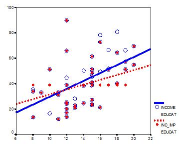
Since most research studies are interested in the relationship among variables, mean imputation is not a good solution. The following graph illustrates this well:

This graph illustrates hypothetical data between X=years of education and Y=annual income in thousands with n=50. The blue circles are the original data, and the solid blue line indicates the best fit regression line for the full data set. The correlation between X and Y is r = .53.
I then randomly deleted 12 observations of income (Y) and substituted the mean. The red dots are the mean-imputed data.
Blue circles with red dots inside them represent non-missing data. Empty Blue circles represent the missing data. If you look across the graph at Y = 39, you will see a row of red dots without blue circles. These represent the imputed values.
The dotted red line is the new best fit regression line with the imputed data. As you can see, it is less steep than the original line. Adding in those red dots pulled it down.
The new correlation is r = .39. That’s a lot smaller that .53.
The real relationship is quite underestimated.
Of course, in a real data set, you wouldn’t notice so easily the bias you’re introducing. This is one of those situations where in trying to solve the lowered sample size, you create a bigger problem.
One note: if X were missing instead of Y, mean substitution would artificially inflate the correlation.
In other words, you’ll think there is a stronger relationship than there really is. That’s not good either. It’s not reproducible and you don’t want to be overstating real results.
This solution that is so good at preserving unbiased estimates for the mean isn’t so good for unbiased estimates of relationships.
Problem #2: Mean Imputation Leads to An Underestimate of Standard Errors
A second reason is applies to any type of single imputation. Any statistic that uses the imputed data will have a standard error that’s too low.
In other words, yes, you get the same mean from mean-imputed data that you would have gotten without the imputations. And yes, there are circumstances where that mean is unbiased. Even so, the standard error of that mean will be too small.
Because the imputations are themselves estimates, there is some error associated with them. But your statistical software doesn’t know that. It treats it as real data.
Ultimately, because your standard errors are too low, so are your p-values. Now you’re making Type I errors without realizing it.
That’s not good.
A better approach? There are two: Multiple Imputation or Full Information Maximum Likelihood.
I’m sure I don’t need to explain to you all the problems that occur as a result of missing data. Anyone who has dealt with missing data—that means everyone who has ever worked with real data—knows about the loss of power and sample size, and the potential bias in your data that comes with listwise deletion.

Listwise deletion is the default method for dealing with missing data in most statistical software packages. It simply means excluding from the analysis any cases with data missing on any variables involved in the analysis.
A very simple, and in many ways appealing, method devised to (more…)
There are many ways to approach missing data. The most common, I  believe, is to ignore it. But making no choice means that your statistical software is choosing for you.
Most of the time, your software is choosing listwise deletion. Listwise deletion may or may not be a bad choice, depending on why and how much data are missing.
Another common approach among those who are paying attention is imputation. Imputation simply means replacing the missing values with an estimate, then analyzing the full data set as if the imputed values were actual observed values.
How do you choose that estimate? The following are common methods: (more…)


