There is something about interactions that is incredibly confusing.
An interaction between two predictor variables means that one predictor variable affects a third variable differently at different values of the other predictor.
How you understand that interaction depends on many things, including:
- Whether one, or both, of the predictor variables is categorical or numerical
- How each of those variables is coded (specifically, whether each categorical variable is dummy or effect coded and whether numerical variables are centered)
- Whether it’s a two-way or three-way interaction
- Whether there is a directionality to the interaction (moderation) or not
Sometimes you need to get pretty sophisticated in your coding, in the output you ask for, and in writing out regression equations.
In this webinar, we’ll examine how to put together and break apart output to understand what your interaction is telling you.
Note: This training is an exclusive benefit to members of the Statistically Speaking Membership Program and part of the Stat’s Amore Trainings Series. Each Stat’s Amore Training is approximately 90 minutes long.
About the Instructor

Karen Grace-Martin helps statistics practitioners gain an intuitive understanding of how statistics is applied to real data in research studies.
She has guided and trained researchers through their statistical analysis for over 15 years as a statistical consultant at Cornell University and through The Analysis Factor. She has master’s degrees in both applied statistics and social psychology and is an expert in SPSS and SAS.
Not a Member Yet?
It’s never too early to set yourself up for successful analysis with support and training from expert statisticians.
Just head over and sign up for Statistically Speaking.
You'll get access to this training webinar, 130+ other stats trainings, a pathway to work through the trainings that you need — plus the expert guidance you need to build statistical skill with live Q&A sessions and an ask-a-mentor forum.
MANOVA is the multivariate (meaning multiple dependent variables) version of ANOVA, but there are many misconceptions about it.
In this webinar, you’ll learn:
- When to use MANOVA and when you’d be better off using individual ANOVAs
- How to follow up the overall MANOVA results to interpret
- What those strange statistics mean — Wilk’s lambda, Roy’s Greatest Root (hint — it’s not a carrot)
- Its relationship to discriminant analysis
Note: This training is an exclusive benefit to members of the Statistically Speaking Membership Program and part of the Stat’s Amore Trainings Series. Each Stat’s Amore Training is approximately 90 minutes long.
About the Instructor
Karen Grace-Martin helps statistics practitioners gain an intuitive understanding of how statistics is applied to real data in research studies.
She has guided and trained researchers through their statistical analysis for over 15 years as a statistical consultant at Cornell University and through The Analysis Factor. She has master’s degrees in both applied statistics and social psychology and is an expert in SPSS and SAS.
Not a Member Yet?
It’s never too early to set yourself up for successful analysis with support and training from expert statisticians.
Just head over and sign up for Statistically Speaking.
You'll get access to this training webinar, 130+ other stats trainings, a pathway to work through the trainings that you need — plus the expert guidance you need to build statistical skill with live Q&A sessions and an ask-a-mentor forum.
In all linear regression models, the intercept has the same definition: the mean of the response, Y, when all predictors, all X = 0.
But “when all X=0” has different implications, depending on the scale on which each X is measured and on which terms are included in the model.
So let’s specifically discuss the meaning of the intercept in some common models: (more…)
Hierarchical regression is a very common approach to model building that allows you to see the incremental contribution to a model of sets of predictor variables.
Popular for linear regression in many fields, the approach can be used in any type of regression model — logistic regression, linear mixed models, or even ANOVA.
In this webinar, we’ll go over the concepts and steps, and we’ll look at how it can be useful in different contexts.
Note: This training is an exclusive benefit to members of the Statistically Speaking Membership Program and part of the Stat’s Amore Trainings Series. Each Stat’s Amore Training is approximately 90 minutes long.
About the Instructor
Karen Grace-Martin helps statistics practitioners gain an intuitive understanding of how statistics is applied to real data in research studies.
She has guided and trained researchers through their statistical analysis for over 15 years as a statistical consultant at Cornell University and through The Analysis Factor. She has master’s degrees in both applied statistics and social psychology and is an expert in SPSS and SAS.
Not a Member Yet?
It’s never too early to set yourself up for successful analysis with support and training from expert statisticians.
Just head over and sign up for Statistically Speaking.
You'll get access to this training webinar, 130+ other stats trainings, a pathway to work through the trainings that you need — plus the expert guidance you need to build statistical skill with live Q&A sessions and an ask-a-mentor forum.
Every statistical software procedure that dummy codes predictor variables uses a default for choosing the reference category.
This default is usually the category that comes first or last alphabetically.
That may or may not be the best category to use, but fortunately you’re not stuck with the defaults.
So if you do choose, which one should you choose? (more…)

In Part 2 of this series, we created two variables and used the lm() command to perform a least squares regression on them, treating one of them as the dependent variable and the other as the independent variable. Here they are again.
height = c(176, 154, 138, 196, 132, 176, 181, 169, 150, 175)
bodymass = c(82, 49, 53, 112, 47, 69, 77, 71, 62, 78)
Today we learn how to obtain useful diagnostic information about a regression model and then how to draw residuals on a plot. As before, we perform the regression.
lm(height ~ bodymass)
Call:
lm(formula = height ~ bodymass)
Coefficients:
(Intercept) bodymass
98.0054 0.9528
Now let’s find out more about the regression. First, let’s store the regression model as an object called mod and then use the summary() command to learn about the regression.
mod <- lm(height ~ bodymass)
summary(mod)
Here is what R gives you.
Call:
lm(formula = height ~ bodymass)
Residuals:
Min 1Q Median 3Q Max
-10.786 -8.307 1.272 7.818 12.253
Coefficients:
Estimate Std. Error t value Pr(>|t|)
(Intercept) 98.0054 11.7053 8.373 3.14e-05 ***
bodymass 0.9528 0.1618 5.889 0.000366 ***
Signif. codes: 0 ‘***’ 0.001 ‘**’ 0.01 ‘*’ 0.05 ‘.’ 0.1 ‘ ’ 1
Residual standard error: 9.358 on 8 degrees of freedom
Multiple R-squared: 0.8126, Adjusted R-squared: 0.7891
F-statistic: 34.68 on 1 and 8 DF, p-value: 0.0003662
R has given you a great deal of diagnostic information about the regression. The most useful of this information are the coefficients themselves, the Adjusted R-squared, the F-statistic and the p-value for the model.
Now let’s use R’s predict() command to create a vector of fitted values.
regmodel <- predict(lm(height ~ bodymass))
regmodel
Here are the fitted values:
1 2 3 4 5 6 7 8 9 10
176.1334 144.6916 148.5027 204.7167 142.7861 163.7472 171.3695 165.6528 157.0778 172.3222
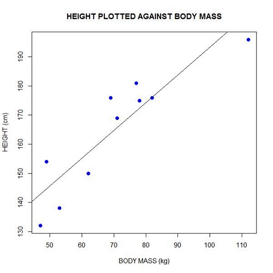
Now let’s plot the data and regression line again.
plot(bodymass, height, pch = 16, cex = 1.3, col = "blue", main = "HEIGHT PLOTTED AGAINST BODY MASS", xlab = "BODY MASS (kg)", ylab = "HEIGHT (cm)")
abline(lm(height ~ bodymass))
We can plot the residuals using R’s for loop and a subscript k that runs from 1 to the number of data points. We know that there are 10 data points, but if we do not know the number of data we can find it using the length() command on either the height or body mass variable.
npoints <- length(height)

npoints
[1] 10
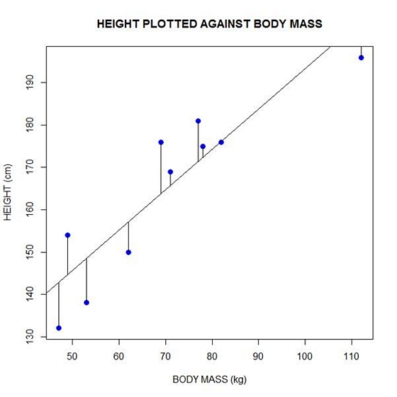
Now let’s implement the loop and draw the residuals (the differences between the observed data and the corresponding fitted values) using the lines() command. Note the syntax we use to draw in the residuals.
for (k in 1: npoints) lines(c(bodymass[k], bodymass[k]), c(height[k], regmodel[k]))
Here is our plot, including the residuals.
In part 4 we will look at more advanced aspects of regression models and see what R has to offer.
About the Author: David Lillis has taught R to many researchers and statisticians. His company, Sigma Statistics and Research Limited, provides both on-line instruction and face-to-face workshops on R, and coding services in R. David holds a doctorate in applied statistics.
See our full R Tutorial Series and other blog posts regarding R programming.