R Is Not So Hard! A Tutorial, Part 3: Regressions and Plots

by David Lillis, Ph.D.

In Part 2 of this series, we created two variables and used the lm() command to perform a least squares regression on them, treating one of them as the dependent variable and the other as the independent variable. Here they are again.

height = c(176, 154, 138, 196, 132, 176, 181, 169, 150, 175)

bodymass = c(82, 49, 53, 112, 47, 69, 77, 71, 62, 78)

Today we learn how to obtain useful diagnostic information about a regression model and then how to draw residuals on a plot. As before, we perform the regression.

lm(height ~ bodymass)
Call:
lm(formula = height ~ bodymass)

Coefficients:
(Intercept)     bodymass 
    98.0054       0.9528  

Now let’s find out more about the regression. First, let’s store the regression model as an object called mod and then use the summary() command to learn about the regression.

mod <-  lm(height ~ bodymass)

summary(mod)

Here is what R gives you.

Call:
lm(formula = height ~ bodymass)
Residuals:
    Min      1Q  Median      3Q     Max 
-10.786  -8.307   1.272   7.818  12.253 

Coefficients:
            Estimate Std. Error t value Pr(>|t|)    
(Intercept)  98.0054    11.7053   8.373 3.14e-05 ***
bodymass      0.9528     0.1618   5.889 0.000366 ***

Signif. codes:  0 ‘***’ 0.001 ‘**’ 0.01 ‘*’ 0.05 ‘.’ 0.1 ‘ ’ 1

Residual standard error: 9.358 on 8 degrees of freedom
Multiple R-squared:  0.8126,    Adjusted R-squared:  0.7891
F-statistic: 34.68 on 1 and 8 DF,  p-value: 0.0003662

R has given you a great deal of diagnostic information about the regression. The most useful of this information are the coefficients themselves, the Adjusted R-squared, the F-statistic and the p-value for the model.

Now let’s use R’s predict() command to create a vector of fitted values.

regmodel <- predict(lm(height ~ bodymass))

regmodel

Here are the fitted values:

    1        2        3        4        5        6        7        8        9       10 
176.1334 144.6916 148.5027 204.7167 142.7861 163.7472 171.3695 165.6528 157.0778 172.3222

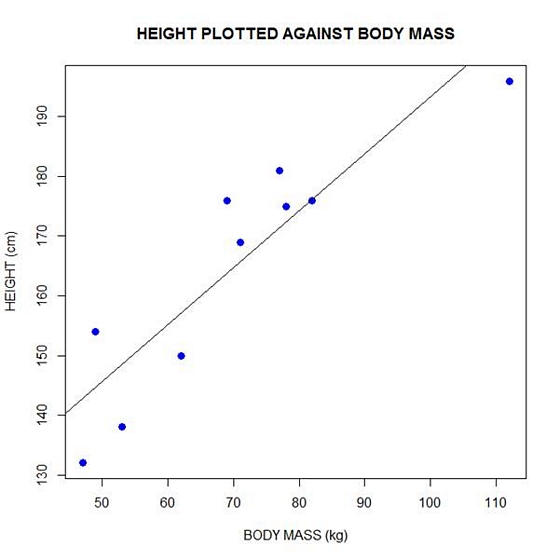
Now let’s plot the data and regression line again.

plot(bodymass, height, pch = 16, cex = 1.3, col = "blue", main = "HEIGHT PLOTTED AGAINST BODY MASS", xlab = "BODY MASS (kg)", ylab = "HEIGHT (cm)")
 
                  abline(lm(height ~ bodymass)) 

We can enhance this plot using various arguments within the

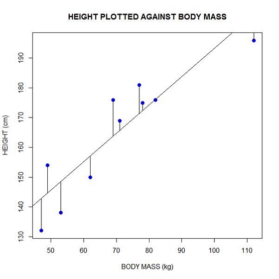
We can plot the residuals using R’s for loop and a subscript k that runs from 1 to the number of data points. We know that there are 10 data points, but if we do not know the number of data we can find it using the length() command on either the height or body mass variable.

npoints <- length(height)
npoints
[1] 10

Now let’s implement the loop and draw the residuals (the differences between the observed data and the corresponding fitted values) using the lines() command. Note the syntax we use to draw in the residuals.

for (k in 1: npoints)  lines(c(bodymass[k], bodymass[k]), c(height[k], regmodel[k]))

Here is our plot, including the residuals.

Next time we will look at more advanced aspects of regression models and see what R has to offer.

See our full R Tutorial Series and other blog posts regarding R programming.


About the Author: David Lillis has taught R to many researchers and statisticians. His company, Sigma Statistics and Research Limited, provides both on-line instruction and face-to-face workshops on R, and coding services in R. David holds a doctorate in applied statistics.

Tagged as: Linear Regression