Linear Models in R: Plotting Regression Lines

by David Lillis, Ph.D.

Today let’s re-create two variables and see how to plot them and include a regression line. We take height to be a variable that describes the heights (in cm) of ten people. Copy and paste the following code to the R command line to create this variable.

height <- c(176, 154, 138, 196, 132, 176, 181, 169, 150, 175)

Now let’s take bodymass to be a variable that describes the masses (in kg) of the same ten people. Copy and paste the following code to the R command line to create the bodymass variable.

bodymass <- c(82, 49, 53, 112, 47, 69, 77, 71, 62, 78)

Both variables are now stored in the R workspace. To view them, enter:

height
 [1] 176 154 138 196 132 176 181 169 150 175

bodymass
 [1] 82 49 53 112 47 69 77 71 62 78

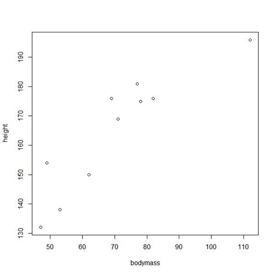
We can now create a simple plot of the two variables as follows:

plot(bodymass, height)

We can enhance this plot using various arguments within the plot() command. Copy and paste the following code into the R workspace:

plot(bodymass, height, pch = 16, cex = 1.3, col = "blue", main = "HEIGHT PLOTTED AGAINST BODY MASS", xlab = "BODY MASS (kg)", ylab = "HEIGHT (cm)")

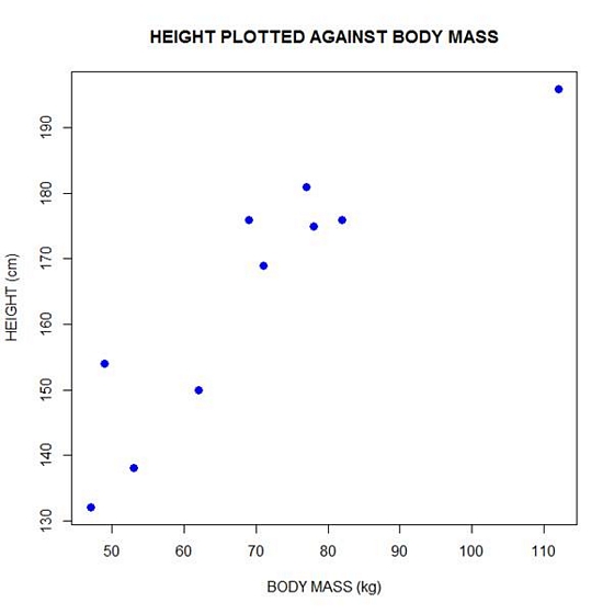
In the above code, the syntax pch = 16 creates solid dots, while cex = 1.3 creates dots that are 1.3 times bigger than the default (where cex = 1). More about these commands later.

Now let’s perform a linear regression using lm() on the two variables by adding the following text at the command line:

lm(height ~ bodymass)
Call:
lm(formula = height ~ bodymass)
Coefficients:
(Intercept)     bodymass
    98.0054       0.9528

We see that the intercept is 98.0054 and the slope is 0.9528. By the way – lm stands for “linear model”.

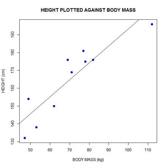
Finally, we can add a best fit line (regression line) to our plot by adding the following text at the command line:

abline(98.0054, 0.9528)

Another line of syntax that will plot the regression line is:

abline(lm(height ~ bodymass))

In the next blog post, we will look again at regression.

See our full R Tutorial Series and other blog posts regarding R programming.

About the Author: David Lillis has taught R to many researchers and statisticians. His company, Sigma Statistics and Research Limited, provides both on-line instruction and face-to-face workshops on R, and coding services in R. David holds a doctorate in applied statistics.

Four Critical Steps in Building Linear Regression Models

While you’re worrying about which predictors to enter, you might be missing issues that have a big impact your analysis. This training will help you achieve more accurate results and a less-frustrating model building experience.

Take Me to The Video!