 In our last post, we calculated Pearson and Spearman correlation coefficients in R and got a surprising result.
So let’s investigate the data a little more with a scatter plot.
We use the same version of the data set of tourists. We have data on tourists from different nations, their gender, number of children, and how much they spent on their trip.
Again we copy and paste the following array into R.
M <- structure(list(COUNTRY = structure(c(3L, 3L, 3L, 3L, 1L, 3L, 2L, 3L, 1L, 3L, 3L, 1L, 2L, 2L, 3L, 3L, 3L, 2L, 3L, 1L, 1L, 3L,

1L, 2L), .Label = c("AUS", "JAPAN", "USA"), class = "factor"),GENDER = structure(c(2L, 1L, 2L, 2L, 1L, 2L, 1L, 2L, 1L, 2L, 2L, 1L, 1L, 1L, 1L, 2L, 1L, 1L, 2L, 2L, 1L, 1L, 1L, 2L), .Label = c("F", "M"), class = "factor"), CHILDREN = c(2L, 1L, 3L, 2L, 2L, 3L, 1L, 0L, 1L, 0L, 1L, 2L, 2L, 1L, 1L, 1L, 0L, 2L, 1L, 2L, 4L, 2L, 5L, 1L), SPEND = c(8500L, 23000L, 4000L, 9800L, 2200L, 4800L, 12300L, 8000L, 7100L, 10000L, 7800L, 7100L, 7900L, 7000L, 14200L, 11000L, 7900L, 2300L, 7000L, 8800L, 7500L, 15300L, 8000L, 7900L)), .Names = c("COUNTRY", "GENDER", "CHILDREN", "SPEND"), class = "data.frame", row.names = c(NA, -24L))
 M

attach(M)
plot(CHILDREN, SPEND)
(more…)
Let’s use R to explore bivariate relationships among variables.
Part 7 of this series showed how to do a nice bivariate plot, but it’s also useful to have a correlation statistic.
We use a new version of the data set we used in Part 20 of tourists from different nations, their gender, and number of children. Here, we have a new variable – the amount of money they spend while on vacation.
First, if the data object (A) for the previous version of the tourists data set is present in your R workspace, it is a good idea to remove it because it has some of the same variable names as the data set that you are about to read in. We remove A as follows:
rm(A)
Removing the object A ensures no confusion between different data objects that contain variables with similar names.
Now copy and paste the following array into R.
M <- structure(list(COUNTRY = structure(c(3L, 3L, 3L, 3L, 1L, 3L, 2L, 3L, 1L, 3L, 3L, 1L, 2L, 2L, 3L, 3L, 3L, 2L, 3L, 1L, 1L, 3L,

1L, 2L), .Label = c("AUS", "JAPAN", "USA"), class = "factor"),GENDER = structure(c(2L, 1L, 2L, 2L, 1L, 2L, 1L, 2L, 1L, 2L, 2L, 1L, 1L, 1L, 1L, 2L, 1L, 1L, 2L, 2L, 1L, 1L, 1L, 2L), .Label = c("F", "M"), class = "factor"), CHILDREN = c(2L, 1L, 3L, 2L, 2L, 3L, 1L, 0L, 1L, 0L, 1L, 2L, 2L, 1L, 1L, 1L, 0L, 2L, 1L, 2L, 4L, 2L, 5L, 1L), SPEND = c(8500L, 23000L, 4000L, 9800L, 2200L, 4800L, 12300L, 8000L, 7100L, 10000L, 7800L, 7100L, 7900L, 7000L, 14200L, 11000L, 7900L, 2300L, 7000L, 8800L, 7500L, 15300L, 8000L, 7900L)), .Names = c("COUNTRY", "GENDER", "CHILDREN", "SPEND"), class = "data.frame", row.names = c(NA, -24L))
 M

attach(M)
Do tourists with greater numbers of children spend more? Let’s calculate the correlation between CHILDREN and SPEND, using the cor() function.
R <- cor(CHILDREN, SPEND)

[1] -0.2612796
We have a weak correlation, but it’s negative! Tourists with a greater number of children tend to spend less rather than more!
(Even so, we’ll plot this in our next post to explore this unexpected finding).
We can round to any number of decimal places using the round() command.
round(R, 2)

[1] -0.26
The percentage of shared variance (100*r2) is:
100 * (R**2)

[1] 6.826704
To test whether your correlation coefficient differs from 0, use the cor.test() command.
cor.test(CHILDREN, SPEND)

 Pearson's product-moment correlation

data: CHILDREN and SPEND

t = -1.2696, df = 22, p-value = 0.2175

alternative hypothesis: true correlation is not equal to 0

95 percent confidence interval:

-0.6012997 0.1588609

sample estimates:

cor

-0.2612796
The cor.test() command returns the correlation coefficient, but also gives the p-value for the correlation. In this case, we see that the correlation is not significantly different from 0 (p is approximately 0.22).
Of course we have only a few values of the variable CHILDREN, and this fact will influence the correlation. Just how many values of CHILDREN do we have? Can we use the levels() command directly? (Recall that the term “level” has a few meanings in statistics, once of which is the values of a categorical variable, aka “factor“).
levels(CHILDREN)

NULL
R does not recognize CHILDREN as a factor. In order to use the levels() command, we must turn CHILDREN into a factor temporarily, using as.factor().
levels(as.factor(CHILDREN))

[1] "0" "1" "2" "3" "4" "5"
So we have six levels of CHILDREN. CHILDREN is a discrete variable without many values, so a Spearman correlation can be a better option. Let’s see how to implement a Spearman correlation:
cor(CHILDREN, SPEND, method ="spearman")

[1] -0.3116905
We have obtained a similar but slightly different correlation coefficient estimate because the Spearman correlation is indeed calculated differently than the Pearson.
Why not plot the data? We will do so in our next post.
About the Author: David Lillis has taught R to many researchers and statisticians. His company, Sigma Statistics and Research Limited, provides both on-line instruction and face-to-face workshops on R, and coding services in R. David holds a doctorate in applied statistics.
See our full R Tutorial Series and other blog posts regarding R programming.
Sometimes when you’re learning a new stat software package, the most frustrating part is not knowing how to do very basic things. This is especially frustrating if you already know how to do them in some other software.
Let’s look at some basic but very useful commands that are available in R.
We will use the following data set of tourists from different nations, their gender and numbers of children. Copy and paste the following array into R.
A <- structure(list(NATION = structure(c(3L, 3L, 3L, 1L, 3L, 2L, 3L,
1L, 3L, 3L, 1L, 2L, 2L, 3L, 3L, 3L, 2L), .Label = c("CHINA",
"GERMANY", "FRANCE"), class = "factor"), GENDER = structure(c(1L,
2L, 2L, 1L, 2L, 1L, 2L, 1L, 2L, 2L, 1L, 1L, 1L, 1L, 2L, 1L, 1L
), .Label = c("F", "M"), class = "factor"), CHILDREN = c(1L,
3L, 2L, 2L, 3L, 1L, 0L, 1L, 0L, 1L, 2L, 2L, 1L, 1L, 1L, 0L, 2L
)), .Names = c("NATION", "GENDER", "CHILDREN"), row.names = 2:18, class = "data.frame")
Want to check that R read the variables correctly? We can look at the first 3 rows using the head() command, as follows:
head(A, 3)
  NATION   GENDER   CHILDREN
2 FRANCE      F        1
3 FRANCE      M        3
4 FRANCE      M        2
Now we look at the last 4 rows using the tail() command:
tail(A, 4)
    NATION   GENDER  CHILDREN
15  FRANCE      F        1
16  FRANCE      M        1
17  FRANCE      F        0
18 GERMANY      F        2
Now we find the number of rows and number of columns using nrow() and ncol().
nrow(A)
[1] 17

ncol(A)
[1] 3
So we have 17 rows (cases) and three columns (variables). These functions look very basic, but they turn out to be very useful if you want to write R-based software to analyse data sets of different dimensions.
Now let’s attach A and check for the existence of particular data.
attach(A)
As you may know, attaching a data object makes it possible to refer to any variable by name, without having to specify the data object which contains that variable.
Does the USA appear in the NATION variable? We use the any() command and put USA inside quotation marks.
any(NATION == "USA")
[1] FALSE
Clearly, we do not have any data pertaining to the USA.
What are the values of the variable NATION?
levels(NATION)
[1] "CHINA"   "GERMANY" "FRANCE"
How many non-missing observations do we have in the variable NATION?
length(NATION)
[1] 17
OK, but how many different values of NATION do we have?
length(levels(NATION))
[1] 3
We have three different values.
Do we have tourists with more than three children? We use the any() command to find out.
any(CHILDREN > 3)
[1] FALSE
None of the tourists in this data set have more than three children.
Do we have any missing data in this data set?
In R, missing data is indicated in the data set with NA.
any(is.na(A))
[1] FALSE
We have no missing data here.
Which observations involve FRANCE? We use the which() command to identify the relevant indices, counting column-wise.
which(A == "FRANCE")
[1]  1  2  3  5  7  9 10 14 15 16
How many observations involve FRANCE? We wrap the above syntax inside the length() command to perform this calculation.
length(which(A == "FRANCE"))
[1] 10
We have a total of ten such observations.
That wasn’t so hard! In our next post we will look at further analytic techniques in R.
About the Author: David Lillis has taught R to many researchers and statisticians. His company, Sigma Statistics and Research Limited, provides both on-line instruction and face-to-face workshops on R, and coding services in R. David holds a doctorate in applied statistics.
See our full R Tutorial Series and other blog posts regarding R programming.
Smoothing can assist data analysis by highlighting important trends and revealing long term movements in time series that otherwise can be hard to see.
Many data smoothing techniques have been developed, each of which may be useful for particular kinds of data and in specific applications. David will give an introductory overview of the most common smoothing methods, and will show examples of their use. He will cover moving averages, exponential smoothing, the Kalman Filter, low-pass filters, high pass filters, LOWESS and smoothing splines.
This presentation is pitched towards those who may use smoothing techniques during the course of their analytic work, but who have little familiarity with the techniques themselves. David will avoid the underpinning mathematical and statistical methods, but instead will focus on providing a clear understanding of what each technique is about.
Note: This training is an exclusive benefit to members of the Statistically Speaking Membership Program and part of the Stat’s Amore Trainings Series. Each Stat’s Amore Training is approximately 90 minutes long.
(more…)
In my last blog post we fitted a generalized linear model to count data using a Poisson error structure.
We found, however, that there was over-dispersion in the data – the variance was larger than the mean in our dependent variable.
(more…)
In my last couple of articles (Part 4, Part 5), I demonstrated a logistic regression model with binomial errors on binary data in R’s glm() function.
But one of wonderful things about glm() is that it is so flexible. It can run so much more than logistic regression models.
The flexibility, of course, also means that you have to tell it exactly which model you want to run, and how.
In fact, we can use generalized linear models to model count data as well.
In such data the errors may well be distributed non-normally and the variance usually increases with the mean values.
As with binary data, we use the glm() command, but this time we specify a Poisson error distribution and the logarithm as the link function.
The natural log is the default link function for the Poisson error distribution. It works well for count data as it forces all of the predicted values to be positive.
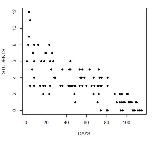
In the following example we fit a generalized linear model to count data using a Poisson error structure. The data set consists of counts of high school students diagnosed with an infectious disease within a period of days from an initial outbreak.
cases <-
structure(list(Days = c(1L, 2L, 3L, 3L, 4L, 4L, 4L, 6L, 7L, 8L,
8L, 8L, 8L, 12L, 14L, 15L, 17L, 17L, 17L, 18L, 19L, 19L, 20L,
23L, 23L, 23L, 24L, 24L, 25L, 26L, 27L, 28L, 29L, 34L, 36L, 36L,
42L, 42L, 43L, 43L, 44L, 44L, 44L, 44L, 45L, 46L, 48L, 48L, 49L,
49L, 53L, 53L, 53L, 54L, 55L, 56L, 56L, 58L, 60L, 63L, 65L, 67L,
67L, 68L, 71L, 71L, 72L, 72L, 72L, 73L, 74L, 74L, 74L, 75L, 75L,
80L, 81L, 81L, 81L, 81L, 88L, 88L, 90L, 93L, 93L, 94L, 95L, 95L,
95L, 96L, 96L, 97L, 98L, 100L, 101L, 102L, 103L, 104L, 105L,
106L, 107L, 108L, 109L, 110L, 111L, 112L, 113L, 114L, 115L),
    Students = c(6L, 8L, 12L, 9L, 3L, 3L, 11L, 5L, 7L, 3L, 8L,
    4L, 6L, 8L, 3L, 6L, 3L, 2L, 2L, 6L, 3L, 7L, 7L, 2L, 2L, 8L,
    3L, 6L, 5L, 7L, 6L, 4L, 4L, 3L, 3L, 5L, 3L, 3L, 3L, 5L, 3L,
    5L, 6L, 3L, 3L, 3L, 3L, 2L, 3L, 1L, 3L, 3L, 5L, 4L, 4L, 3L,
    5L, 4L, 3L, 5L, 3L, 4L, 2L, 3L, 3L, 1L, 3L, 2L, 5L, 4L, 3L,
    0L, 3L, 3L, 4L, 0L, 3L, 3L, 4L, 0L, 2L, 2L, 1L, 1L, 2L, 0L,
    2L, 1L, 1L, 0L, 0L, 1L, 1L, 2L, 2L, 1L, 1L, 1L, 1L, 0L, 0L,
    0L, 1L, 1L, 0L, 0L, 0L, 0L, 0L)), .Names = c("Days", "Students"
), class = "data.frame", row.names = c(NA, -109L))

attach(cases)

head(cases)
    Days Students
1    1      6
2    2      8
3    3     12
4    3      9
5    4      3
6    4      3
The mean and variance are different (actually, the variance is greater). Now we plot the data.
plot(Days, Students, xlab = "DAYS", ylab = "STUDENTS", pch = 16)
Now we fit the glm, specifying the Poisson distribution by including it as the second argument.
model1 <- glm(Students ~ Days, poisson) summary(model1) Call: glm(formula = Students ~ Days, family = poisson) Deviance Residuals: Min 1Q Median 3Q Max -2.00482 -0.85719 -0.09331 0.63969 1.73696 Coefficients: Estimate Std. Error z value Pr(>|z|)
(Intercept)  1.990235   0.083935   23.71   <2e-16 ***
Days        -0.017463   0.001727  -10.11   <2e-16 ***
---
Signif. codes:  0 ‘***’ 0.001 ‘**’ 0.01 ‘*’ 0.05 ‘.’ 0.1 ‘ ’ 1

(Dispersion parameter for poisson family taken to be 1)

    Null deviance: 215.36  on 108  degrees of freedom
Residual deviance: 101.17  on 107  degrees of freedom
AIC: 393.11

Number of Fisher Scoring iterations: 5
The negative coefficient for Days indicates that as days increase, the mean number of students with the disease is smaller.
This coefficient is highly significant (p < 2e-16).
We also see that the residual deviance is greater than the degrees of freedom, so that we have over-dispersion. This means that there is extra variance not accounted for by the model or by the error structure.
This is a very important model assumption, so in my next article we will re-fit the model using quasi poisson errors.
****
See our full R Tutorial Series and other blog posts regarding R programming.
About the Author: David Lillis has taught R to many researchers and statisticians. His company, Sigma Statistics and Research Limited, provides both on-line instruction and face-to-face workshops on R, and coding services in R. David holds a doctorate in applied statistics.