
In Part 2 of this series, we created two variables and used the lm() command to perform a least squares regression on them, treating one of them as the dependent variable and the other as the independent variable. Here they are again.
height = c(176, 154, 138, 196, 132, 176, 181, 169, 150, 175)
bodymass = c(82, 49, 53, 112, 47, 69, 77, 71, 62, 78)
Today we learn how to obtain useful diagnostic information about a regression model and then how to draw residuals on a plot. As before, we perform the regression.
lm(height ~ bodymass)
Call:
lm(formula = height ~ bodymass)
Coefficients:
(Intercept) bodymass
98.0054 0.9528
Now let’s find out more about the regression. First, let’s store the regression model as an object called mod and then use the summary() command to learn about the regression.
mod <- lm(height ~ bodymass)
summary(mod)
Here is what R gives you.
Call:
lm(formula = height ~ bodymass)
Residuals:
Min 1Q Median 3Q Max
-10.786 -8.307 1.272 7.818 12.253
Coefficients:
Estimate Std. Error t value Pr(>|t|)
(Intercept) 98.0054 11.7053 8.373 3.14e-05 ***
bodymass 0.9528 0.1618 5.889 0.000366 ***
Signif. codes: 0 ‘***’ 0.001 ‘**’ 0.01 ‘*’ 0.05 ‘.’ 0.1 ‘ ’ 1
Residual standard error: 9.358 on 8 degrees of freedom
Multiple R-squared: 0.8126, Adjusted R-squared: 0.7891
F-statistic: 34.68 on 1 and 8 DF, p-value: 0.0003662
R has given you a great deal of diagnostic information about the regression. The most useful of this information are the coefficients themselves, the Adjusted R-squared, the F-statistic and the p-value for the model.
Now let’s use R’s predict() command to create a vector of fitted values.
regmodel <- predict(lm(height ~ bodymass))
regmodel
Here are the fitted values:
1 2 3 4 5 6 7 8 9 10
176.1334 144.6916 148.5027 204.7167 142.7861 163.7472 171.3695 165.6528 157.0778 172.3222
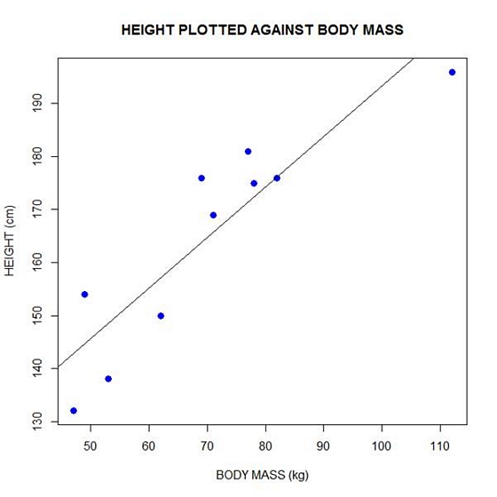
Now let’s plot the data and regression line again.
plot(bodymass, height, pch = 16, cex = 1.3, col = "blue", main = "HEIGHT PLOTTED AGAINST BODY MASS", xlab = "BODY MASS (kg)", ylab = "HEIGHT (cm)")
abline(lm(height ~ bodymass))
We can plot the residuals using R’s for loop and a subscript k that runs from 1 to the number of data points. We know that there are 10 data points, but if we do not know the number of data we can find it using the length() command on either the height or body mass variable.
npoints <- length(height)

npoints
[1] 10
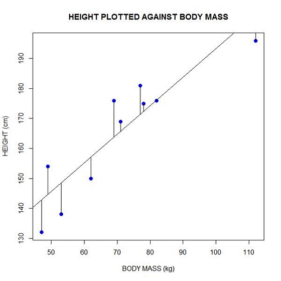
Now let’s implement the loop and draw the residuals (the differences between the observed data and the corresponding fitted values) using the lines() command. Note the syntax we use to draw in the residuals.
for (k in 1: npoints) lines(c(bodymass[k], bodymass[k]), c(height[k], regmodel[k]))
Here is our plot, including the residuals.
In part 4 we will look at more advanced aspects of regression models and see what R has to offer.
About the Author: David Lillis has taught R to many researchers and statisticians. His company, Sigma Statistics and Research Limited, provides both on-line instruction and face-to-face workshops on R, and coding services in R. David holds a doctorate in applied statistics.
See our full R Tutorial Series and other blog posts regarding R programming.
In Part 1 we installed R and used it to create a variable and summarize it using a few simple commands. Today let’s re-create that variable and also create a second variable, and see what we can do with them.
As before, we take height to be a variable that describes the heights (in cm) of ten people. Type the following code to the R command line to create this variable.
height = c(176, 154, 138, 196, 132, 176, 181, 169, 150, 175)
Now let’s take bodymass to be a variable that describes the weight (in kg) of the same ten people. Copy and paste the following code to the R command line to create the bodymass variable.
bodymass = c(82, 49, 53, 112, 47, 69, 77, 71, 62, 78)
Both variables are now stored in the R workspace. To view them, enter:
height bodymass
We can now create a simple plot of the two variables as follows:
plot(bodymass, height)
However, this is a rather simple plot and we can embellish it a little. Type the following code into the R workspace:
plot(bodymass, height, pch = 16, cex = 1.3, col = "red", main = "MY FIRST PLOT USING R", xlab = "Body Mass (kg)", ylab = "HEIGHT (cm)")
[Note: R is very picky about the quotation marks you use. If the font that is displaying this post shows the beginning and ending quotation marks as facing in different directions, it won’t work in R. They both have to look the same–just straight lines. You may have to retype them within R rather than cutting and pasting.]
In the above code, the syntax pch = 16 creates solid dots, while cex = 1.3 creates dots that are 1.3 times bigger than the default (where cex = 1). More about these commands later.
Now let’s perform a linear regression on the two variables by adding the following text at the command line:
lm(height~bodymass)
We see that the intercept is 98.0054 and the slope is 0.9528. By the way – lm stands for “linear model”.
Finally, we can add a best fit line to our plot by adding the following text at the command line:
abline(98.0054, 0.9528)
None of this was so difficult!
In Part 3 we will look again at regression and create more sophisticated plots.
About the Author: David Lillis has taught R to many researchers and statisticians. His company, Sigma Statistics and Research Limited, provides both on-line instruction and face-to-face workshops on R, and coding services in R. David holds a doctorate in applied statistics.
See our full R Tutorial Series and other blog posts regarding R programming.
Two methods for dealing with missing data, vast improvements over traditional approaches, have become available in mainstream statistical software in the last few years.
Both of the methods discussed here require that the data are missing at random–not related to the missing values. If this assumption holds, resulting estimates (i.e., regression coefficients and standard errors) will be unbiased with no loss of power.
The first method is Multiple Imputation (MI). Just like the old-fashioned imputation (more…)
Many of you have heard of R (the R statistics language and environment for scientific and statistical computing and graphics). Perhaps you know that it uses command line input rather than pull-down menus. Perhaps you feel that this makes R hard to use and somewhat intimidating!
OK. Indeed, R has a longer learning curve than other systems, but don’t let that put you off! Once you master the syntax, you have control of an immensely powerful statistical tool.
Actually, much of the syntax is not all that difficult. Don’t believe me? To prove it, let’s look at some syntax for providing summary statistics on a continuous variable. (more…)
Before you run a Cronbach’s alpha or factor analysis on scale items, it’s generally a good idea to reverse code items that are negatively worded so that a high value indicates the same type of response on every item.
So for example let’s say you have 20 items each on a 1 to 7 scale. For most items, a 7 may indicate a positive attitude toward some issue, but for a few items, a 1 indicates a positive attitude.
I want to show you a very quick and easy way to reverse code them using a single command line. This works in any software. (more…)
It seems every editor and her brother these days wants to see standardized effect size statistics reported in journal articles.
For ANOVAs, two of the most popular are Eta-squared and partial Eta-squared. In one way ANOVAs, they come out the same, but in more complicated models, their values, and their meanings differ.
SPSS only reports partial Eta-squared, and in earlier versions of the software it was (unfortunately) labeled Eta-squared. More recent versions have fixed the label, but still don’t offer Eta-squared as an option.
Luckily Eta-squared is very simple to calculate yourself based on the sums of squares in your ANOVA table. I’ve written another blog post with all the formulas. You can (more…)