
An “estimation command” in Stata is a generic term used for a command that runs a statistical model. Examples are regress, ANOVA, Poisson, logit, and mixed.
Stata has more than 100 estimation commands.
Creating the “best” model requires trying alternative models. There are a number of different model building approaches, but regardless of the strategy you take, you’re going to need to compare them.
Running all these models can generate a fair amount of output to compare and contrast. How can you view and keep track of all of the results?
You could scroll through the results window on your screen. But this method makes it difficult to compare differences.
You could copy and paste the results into a Word document or spreadsheet. Or better yet use the “esttab” command to output your results. But both of these require a number of time consuming steps.
But Stata makes it easy: my suggestion is to use the post-estimation command “estimates”.
What is a post-estimation command? A post-estimation command analyzes the stored results of an estimation command (regress, ANOVA, etc).
As long as you give each model a different name you can store countless results (Stata stores the results as temp files). You can then use post-estimation commands to dig deeper into the results of that specific estimation.
Here is an example. I will run four regression models to examine the impact several factors have on one’s mental health (Mental Composite Score). I will then store the results of each one.
regress MCS weeks_unemployed i.marital_status
estimates store model_1
regress MCS weeks_unemployed i.marital_status kids_in_house
estimates store model_2
regress MCS weeks_unemployed i.marital_status kids_in_house religious_attend
estimates store model_3
regress MCS weeks_unemployed i.marital_status kids_in_house religious_attend income
estimates store model_4
To view the results of the four models in one table my code can be as simple as:
estimates table model_1 model_2 model_3 model_4
But I want to format it so I use the following:
estimates table model_1 model_2 model_3 model_4, varlabel varwidth(25) b(%6.3f) /// star(0.05 0.01 0.001) stats(N r2_a)
Here are my results:
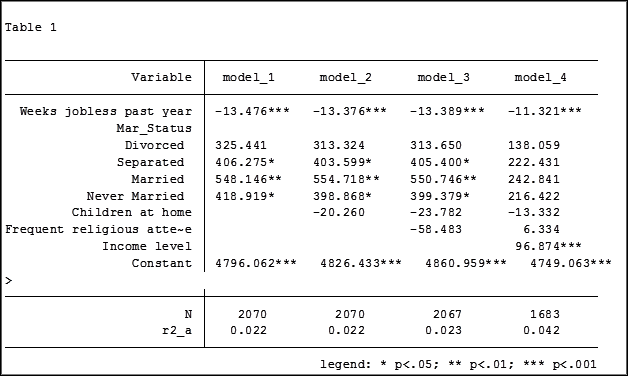
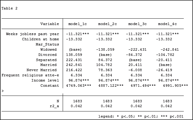
My base category for marital status was “widowed”. Is “widowed” the base category I want to use in my final analysis? I can easily re-run model 4, using a different reference group base category each time.
Putting the results into one table will make it easier for me to determine which category to use as the base.
Note in table 1 the size of the samples have changed from model 2 (2,070) to model 3 (2,067) to model 4 (1,682). In the next article we will explore how to use post-estimation data to use the same sample for each model.
Jeff Meyer is a statistical consultant with The Analysis Factor, a stats mentor for Statistically Speaking membership, and a workshop instructor. Read more about Jeff here.
Stata has perhaps the best support resources of any statistical software
to help you prepare and analyze your data. These resources are helpful
for all skill levels, from beginners to advanced users.
For just about any Stata command, there are FAQs, text books, Stata
Journal articles, and third party add-ons, not to mention the built in
help page.
Even these help pages are detailed — broken into subsections;
description, syntax, menu, and examples.
Learning the nuances of the resources and how to quickly find the one
you need will help you create accurate analysis in significantly less time.
We will start by exploring commands with few options such as *generate*
and *navigate* to commands with many options such as *egen.*
**
This free one hour webinar will be packed full of information that will
help reduce those frustrating moments that we all experience when using
software.
Title: How to Benefit from Stata’s Bountiful Help Resources
Date: Thurs Dec 17, 2015
Time: 2:00pm EST
Presenter: Jeff Meyer
This webinar has already taken place. Please sign up below to get access to the video recording.
Share the free December 2015 webinar with others!


Jeff Meyer is a statistical consultant with The Analysis Factor, a stats mentor for Statistically Speaking membership, and a workshop instructor. Read more about Jeff here.
I recently opened a very large data set titled “1998 California Work and Health Survey” compiled by the Institute for Health Policy Studies at the University of California, San Francisco. There are 1,771 observations and 345 variables. (more…)
Have you ever worked with a data set that had so many observations and/or variables that you couldn’t see the forest for the trees? You would like to extract some simple information but you can’t quite figure out how to do it.
Get to know Stata’s collapse command–it’s your new friend. Collapse allows you to convert your current data set to a much smaller data set of means, medians, maximums, minimums, count or percentiles (your choice of which percentile).
Let’s take a look at an example. I’m currently looking at a longitudinal data set filled with economic data on all 67 counties in Alabama. The time frame is in decades, from 1960 to 2000. Five time periods by 67 counties give me a total of 335 observations.
What if I wanted to see some trend information, such as the total population and jobs per decade for all of Alabama? I just want a simple table to see my results as well as a graph. I want results that I can copy and paste into a Word document.
Here’s my code:
preserve

collapse (sum) Pop Jobs, by(year)

graph twoway (line Pop year) (line Jobs year), ylabel(, angle(horizontal))

list
And here is my output:
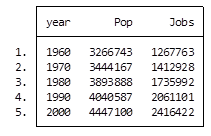
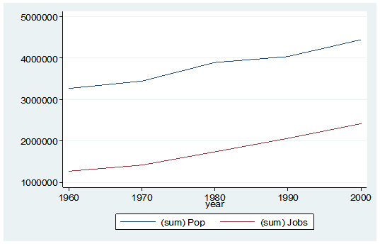
By starting my code with the preserve command it brings my data set back to its original state after providing me with the results I want.
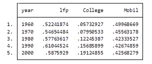
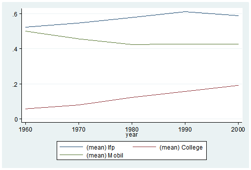
What if I want to look at variables that are in percentages, such as percent of college graduates, mobility and labor force participation rate (lfp)? In this case I don’t want to sum the values because they are in percent.
Calculating the mean would give equal weighting to all counties regardless of size.
Fortunately Stata gives you a very simple way to weight your data based on frequency. You have to determine which variable to use. In this situation I will use the population variable.
Here’s my coding and results:
Preserve

collapse (mean) lfp College Mobil [fw=Pop], by(year)

graph twoway (line lfp year) (line College year) (line Mobil year), ylabel(, angle(horizontal))

list
It’s as easy as that. This is one of the five tips and tricks I’ll be discussing during the free Stata webinar on Wednesday, July 29th.
Jeff Meyer is a statistical consultant with The Analysis Factor, a stats mentor for Statistically Speaking membership, and a workshop instructor. Read more about Jeff here.
One of Stata’s incredibly useful abilities is to temporarily store calculations from commands.
Why is this so useful? (more…)
For my first assignment using Stata, I spent four or five hours trying to present my output in a “professional” form. The most creative method I heard about in class the next day was to copy the contents into Excel, create page breaks, and then copy into Word.
SPSS makes it so easy to copy tables and graphs into another document. Why can’t Stata be easy?
Anyone who has used Stata has gone through this and many of you still are. No worries, help is on the way! (more…)