R-Squared for Mixed Effects Models

When learning about linear models —that is, regression, ANOVA, and similar techniques—we are taught to calculate an R². The R² has the following useful properties:

• The range is limited to [0,1], so we can easily judge how relatively large it is.
• It is standardized, meaning its value does not depend on the scale of the variables involved in the analysis.
• The interpretation is pretty clear: It is the proportion of variability in the outcome that can be explained by the independent variables in the model.

The calculation of the R² is also intuitive, once you understand the concepts of variance and prediction. One way to write the formula for R² from a GLM is

where  is an actual individual outcome, is the model-predicted outcome that goes with it, and is the average of all the outcomes.

In this formula, the denominator measures all of the variability in  without considering the model. The numerator E ach  in the numerator represents how much closer the model’s predicted value gets us to the actual outcome than the mean does. Therefore, the fraction is the proportion of all of the variability in the outcome that is explained by the model.

The key to the neatness of this formula is that there are only two sources of variability in a linear model: the fixed effects (“explainable”) and the rest of it, which we often call error (“unexplainable”).

When we try to move to more complicated models, however, defining and agreeing on an R² becomes more difficult. That is especially true with mixed effects models, where there is more than one source of variability (one or more random effects, plus residuals).

These issues, and a solution that many analysts now refer to, are presented in the 2012 article A general and simple method for obtaining R² from generalized linear mixed‐effects models by Nakagawa and Shielzeth (see https://besjournals.onlinelibrary.wiley.com/doi/10.1111/j.2041-210x.2012.00261.x). These authors present two different options for calculating a mixed-effects R², which they call the “marginal” and “conditional” R².

Before describing these formulas, let’s borrow an example study from the Analysis Factor’s workshop “Introduction to Generalized Linear Mixed Models.” Suppose we are trying to predict the weight of a chick, based on its diet and number of days since hatching. Each chick in the data was weighed on multiple days, producing multiple outcomes for a single chick.

This analysis needs to account for the following sources of variability: the “fixed” effects of diet and time, the differences across the chicks (which we would call “random” because the chicks are randomly selected), and the prediction errors that occur when we try to use the model to predict a chick’s exact weight based on its diet and days since hatching.

The marginal R² for LMMs described by Nakagawa and Shielzeth is calculated by

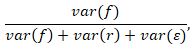
where is the variance of the fixed effects ,  is the variance of the random effect  and is the variance of the model residuals . In the context of the chick example, is the variability explained by diet and days since hatching,  is the variance attributed to differences across chicks, and  is the variability of the errors in individual weight predictions. Together, these three sources of variability add up to the total variability (denominator of the marginal R² equation). Dividing the variance of the fixed effects only by this total variability provides us with a measure of the proportion of variability explained by the fixed effects.

However, this leads to a question: is the fixed effects part of the model the only part that is “explained?” Or is the variation across the chicks, which we have been calling “random,” now also “explained?” For those who would claim that random variability is explained, because it has been separated from residual variability, we calculate the conditional R² for LMMs:

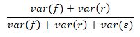
The conditional R² is the proportion of total variance explained through both fixed and random effects.

The article by Nakagawa and Shielzeth goes on to expand these formulas to situations with more than one random variable, and also to the generalized linear mixed effects model (GLMM).

The GLMM versions should be interpreted with the same caution we use with a pseudo R² from a more basic generalized linear model.  Concepts like “residual variability” do not have the same meaning in GLMMs. The article also discusses the advantages and limitations of each of these formulas, and compares their usefulness to other earlier versions of mixed effects R² calculations.

Note that these versions of R² are becoming more common, but are not entirely agreed upon or standard. You will not be able to calculate them directly in standard software. Instead, you need to calculate the components and program the calculation. Importantly, if you choose to report one or both of them, you should not only identify which one you are using, but provide some brief interpretation and a citation of the article.

What is GLMM and When Should You Use It?

When you have multilevel or repeated data and normality just isn't happening, you may need GLMM. Get started learning Generalized Linear Mixed Models and when and how to apply them to your data.

Take Me to The Video!