There are quite a few types of outcome variables that will never meet ordinary linear model’s assumption of normally distributed residuals. A non-normal outcome variable can have normally distribued residuals, but it does need to be continuous, unbounded, and measured on an interval or ratio scale. Categorical outcome variables clearly don’t fit this requirement, so it’s easy to see that an ordinary linear model is not appropriate. Neither do count variables. It’s less obvious, because they are measured on a ratio scale, so it’s easier to think of them as continuous, or close to it. But they’re neither continuous or unbounded, and this really affects assumptions.
Continuous variables measure how much. Count variables measure how many. Count variables can’t be negative—0 is the lowest possible value, and they’re often skewed–so severly that 0 is by far the most common value. And they’re discrete, not continuous. All those jokes about the average family having 1.3 children have a ring of truth in this context.
Count variables often follow a Poisson or one of its related distributions. The Poisson distribution assumes that each count is the result of the same Poisson process—a random process that says each counted event is independent and equally likely. If this count variable is used as the outcome of a regression model, we can use Poisson regression to estimate how predictors affect the number of times the event occurred.
But the Poisson model has very strict assumptions. One that is often violated is that the mean equals the variance. When the variance is too large because there are many 0s as well as a few very high values, the negative binomial model is an extension that can handle the extra variance.
But sometimes it’s just a matter of having too many zeros than a Poisson would predict. In this case, a better solution is often the Zero-Inflated Poisson (ZIP) model. (And when extra variation occurs too, its close relative is the Zero-Inflated Negative Binomial model).
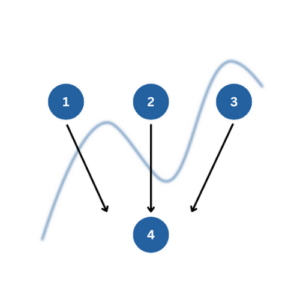
ZIP models assume that some zeros occurred by a Poisson process, but others were not even eligible to have the event occur. So there are two processes at work—one that determines if the individual is even eligible for a non-zero response, and the other that determines the count of that response for eligible individuals.
The tricky part is either process can result in a 0 count. Since you can’t tell which 0s were eligible for a non-zero count, you can’t tell which zeros were results of which process. The ZIP model fits, simultaneously, two separate regression models. One is a logistic or probit model that models the probability of being eligible for a non-zero count. The other models the size of that count.
Both models use the same predictor variables, but estimate their coefficients separately. So the predictors can have vastly different effects on the two processes.
But a ZIP model requires it be theoretically plausible that some individuals are ineligible for a count. For example, consider a count of the number of disciplinary incidents in a day in a youth detention center. True, there may be some youth who would never instigate an incident, but the unit of observation in this case is the center. It is hard to imagine a situation in which a detention center would have no possibility of any incidents, even if they didn’t occur on some days.
Compare that to the number of alcoholic drinks consumed in a day, which could plausibly be fit with a ZIP model. Some participants do drink alcohol, but will have consumed 0 that day, by chance. But others just do not drink alcohol, so will never have a non-zero response. The ZIP model can determine which predictors affect the probability of being an alcohol consumer and which predictors affect how many drinks the consumers consume. They may not be the same predictors for the two models, or they could even have opposite effects on the two processes.
One of the most anxiety-laden questions I get from researchers is whether their analysis is “right.”
I’m always slightly uncomfortable with that word. Often there is no one right analysis.
It’s like finding Mr. or Ms. or Mx. Right. Most of the time, there is not just one Right. But there are many that are clearly Wrong.
But there are characteristics of an analysis that makes it work. Let’s take a look.
What Makes an Analysis Right?
Luckily, what makes an analysis right is easier to define than what makes a person right for you. It pretty much comes down to two things: whether the assumptions of the statistical method are being met and whether the analysis answers the research question.
Assumptions are very important. A test needs to reflect the measurement scale of the variables, the study design, and issues in the data. A repeated measures study design requires a repeated measures analysis. A binary dependent variable requires a categorical analysis method.
If you don’t match the measurement scale of the variables to the appropriate test or model, you’re going to have trouble meeting assumptions. And yes, there are ad-hoc strategies to make assumptions seem more reasonable, like transformations. But these strategies are not a cure-all and you’re better off sticking with an analysis that fits the variables.
But within those general categories of appropriate analysis, there are often many analyses that meet assumptions.
A logistic regression or a chi-square test both handle a binary dependent variable with a single categorical predictor. But a logistic regression can answer more research questions. It can incorporate covariates, directly test interactions, and calculate predicted probabilities. A chi-square test can do none of these.
So you get different information from different tests. They answer different research questions.
An analysis that is correct from an assumptions point of view is useless if it doesn’t answer the research question. A data set can spawn an endless number of statistical tests and models that don’t answer the research question. And you can spend an endless number of days running them.
When to Think about the Analysis
The real bummer is it’s not always clear that the analyses aren’t relevant until you are all done with the analysis and start to write up the research paper.
That’s why writing out the research questions in theoretical and operational terms is the first step of any statistical analysis.
It’s absolutely fundamental.
 And I mean writing them in minute detail. Issues of mediation, interaction, subsetting, control variables, et cetera, should all be blatantly obvious in the research questions.
This is one step where it can be extremely valuable to talk to your statistical consultant. It’s something we do all the time in the Statistically Speaking membership.
Thinking about how to analyze the data before collecting the data can help you from hitting a dead end. It can be very obvious, once you think through the details, that the analysis available to you based on the data won’t answer the research question.
Whether the answer is what you expected or not is a different issue.
So when you are concerned about getting an analysis “right,” clearly define the design, variables, and data issues. And check whatever assumptions you can!
But most importantly, get explicitly clear about what you want to learn from this analysis.
Once you’ve done this, it’s much easier to find the statistical method that answers the research questions and meets assumptions. And if this feels pointless because you don’t know which is the analysis that matches that combination, that’s what we’re here for. Our statistical team at The Analysis Factor can help you with any of these steps.
Yesterday I gave a little quiz about interpreting regression coefficients. Today I’m giving you the answers.
If you want to try it yourself before you see the answers, go here. (It’s truly little, but if you’re like me, you just cannot resist testing yourself).
True or False?
1. When you add an interaction to a regression model, you can still evaluate the main effects of the terms that make up the interaction, just like in ANOVA. (more…)
Here’s a little quiz:
True or False?
1. When you add an interaction to a regression model, you can still evaluate the main effects of the terms that make up the interaction, just like in ANOVA.
2. The intercept is usually meaningless in a regression model. (more…)
Here’s a little tip.
When you construct Dummy Variables, make it easy on yourself to remember which code is which. Heck, if you want to be really nice, make it easy for anyone else who will analyze the data or read the results.
Make the codes inherent in the Dummy variable name.
So instead of a variable named Gender with values of 1=Female and 0=Male, call the variable Female.
Instead of a set of dummy variables named MaritalStatus1 with values of 1=Married and 0=Single, along with MaritalStatus2 with values 1=Divorced and 0=Single, name the same variables Married and Divorced.
And if you’re new to dummy coding, this has the extra bonus of making the dummy coding intuitive. It’s just a set of yes/no variables about all but one of your categories.
Someone who registered for my upcoming Interpreting (Even Tricky) Regression Models workshop asked if the content applies to logistic regression as well.
The short answer: Yes
The long-winded detailed explanation of why this is true and the one caveat:
One of the greatest things about regression models is that they all have the same set up: (more…)


