 In most regression models, there is one response variable and one or more predictors. From the model’s point of view, it doesn’t matter if those predictors are there to predict, to moderate, to explain, or to control. All that matters is that they’re all Xs, on the right side of the equation.
Structural equation modeling, though, is a system of equations. Sure, it can be such a simple system that it has only one equation, but it’s flexible enough to have many.
And when you have many equations, the same variable can be a response variable in one equation and a predictor in another. So the simple response/predictor dichotomy breaks down a bit because you may have only a few variables that are only a predictor or only a response.
But there is still an important and related dichotomy: Exogenous and Endogenous. Let’s take a look at what these are.
The difference between exogenous and endogenous
Endogenous variables are response variables in some equation, anywhere in the model. In other words, if somewhere in the model, there is a one-headed arrow pointed to it, the variable is endogenous.
The final response variable, if there is one, is always endogenous. So are mediators. So are any variables we might otherwise think of as predictors, if some other predictor is affecting their value.
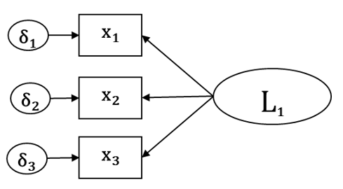
In the following diagram, all the x variables are endogenous.
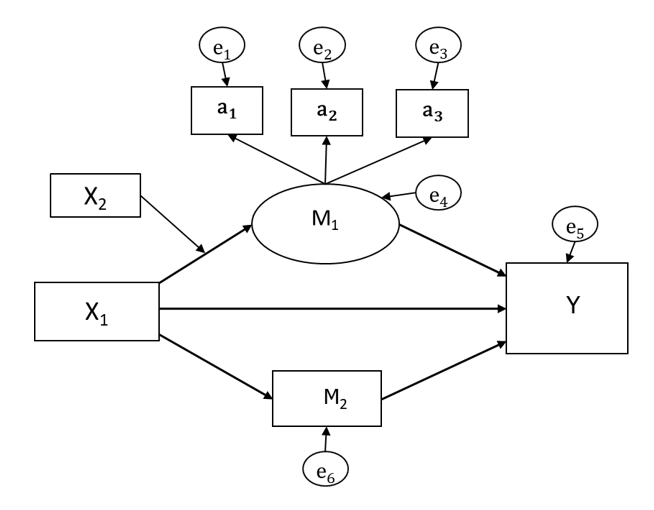
And in this one, we have six endogenous variables: M₁, a₁, a₂, a₃, Y, and M₂.
 Exogenous variables are never, ever response variables. They can be correlated with other variables, so have one end of a two-headed arrow pointed toward them. But never a one-headed arrow.
Why this difference matters
When you make a variable exogenous, you’re assuming there are no other variables causing or affecting that variable. This is a particularly important assumption if you’re making any causal inferences. This can be easy to assume for some variables, like treatments with random assignment or some demographic variables, (like age) but something to consider carefully with observed variables.
The big structural difference between exogenous and endogenous variables is endogenous variables have error terms. In other words, we’re stating that two different things affect their value:
- Other variables, as represented by the arrows pointing to them.
- Random unexplained variance, as represented by the error term.
Exogenous variables don’t have error terms. This means you’re also assuming they’re measured without error. Again, that’s a pretty easy assumption for some variables, like whether someone received the treatment or a placebo. It’s a harder assumption to make for others, like income.
So it’s important for the model, and for you, the modeler, to know whether a variable is exogenous or endogenous. If it’s endogenous, there will be a parameter estimate for the variable’s error variance. If it’s exogenous, there won’t be.
Very often, SEM models are written without these error terms. It’s a shortcut that people use who know there should be an error term there and don’t want to clutter up the diagram.
If you’re still learning SEM, or presenting a model to others who are still learning SEM, I recommend always putting the error terms in. Just for the sake of clarity. If you’re reading someone else’s model, whether that error variance is there or implied, you can always count on the arrows.

Leave a Reply