R Is Not So Hard! A Tutorial, Part 5: Fitting an Exponential Model

by David Lillis, Ph.D.

In Part 3 and Part 4 we used the lm() command to perform least squares regressions. We saw how to check for non-linearity in our data by fitting polynomial models and checking whether they fit the data better than a linear model. Now let’s see how to fit an exponential model in R.

As before, we will use a data set of counts (atomic disintegration events that take place within a radiation source), taken with a Geiger counter at a nuclear plant.

The counts were registered over a 30 second period for a short-lived, man-made radioactive compound. We read in the data and subtract the background count of 623.4 counts per second in order to obtain the counts that pertain to the radio-active source.

Once again, cut and paste the following data into the R workspace.

A <- structure(list(Time = c(0, 1, 2, 4, 6, 8, 9, 10, 11, 12, 13, 
14, 15, 16, 18, 19, 20, 21, 22, 24, 25, 26, 27, 28, 29, 30), 
Counts = c(126.6, 101.8, 71.6, 101.6, 68.1, 62.9, 45.5, 41.9, 
46.3, 34.1, 38.2, 41.7, 24.7, 41.5, 36.6, 19.6, 
22.8, 29.6, 23.5, 15.3, 13.4, 26.8, 9.8, 18.8, 25.9, 19.3)), .Names = c("Time", "Counts"), row.names = c(1L, 2L,
3L, 5L, 7L, 9L, 10L, 11L, 12L, 13L, 14L, 15L, 16L, 17L, 19L, 20L, 21L, 22L, 23L, 25L, 26L, 27L, 28L, 29L, 30L,
31L), class = "data.frame")

Let’s attach the entire dataset so that we can refer to all variables directly by name.

attach(A)

names(A)

Let’s see if an exponential function fits the data even better than a quadratic. We set up a grid of points and superpose the exponential function on the previous plot. An exponential function in the Time variable can be treated as a model of the log of the Counts variable.

exponential.model <- lm(log(Counts)~ Time)

summary(exponential.model)

R returns the following output:

Call:
lm(formula = log(Counts) ~ Time)

Residuals:
     Min       1Q   Median       3Q     Max 
-0.54715 -0.17618 0.02855 0.18850 0.55254 

Coefficients:
             Estimate Std. Error t value Pr(>|t|)   
(Intercept) 4.555249   0.111690   40.78 < 2e-16 ***
Time       -0.063915   0.006158 -10.38 2.36e-10 ***
---
Signif. codes: 0 ‘***’ 0.001 ‘**’ 0.01 ‘*’ 0.05 ‘.’ 0.1 ‘ ’ 1

Residual standard error: 0.2814 on 24 degrees of freedom
Multiple R-squared: 0.8178,   Adjusted R-squared: 0.8102 
F-statistic: 107.7 on 1 and 24 DF, p-value: 2.362e-10

This model is pretty good, though it explains about 81% of the variance by comparison with the 89% explained by the quadratic model. Let’s plot it on a grid of time values from 0 to 30 in intervals of 0.1 seconds.

timevalues <- seq(0, 30, 0.1)

Counts.exponential2 <- exp(predict(exponential.model,list(Time=timevalues)))

plot(Time, Counts,pch=16)

lines(timevalues, Counts.exponential2,lwd=2, col = "red", xlab = "Time (s)", ylab = "Counts")

Note that we used the exponential of the predicted values in the second line of syntax above.

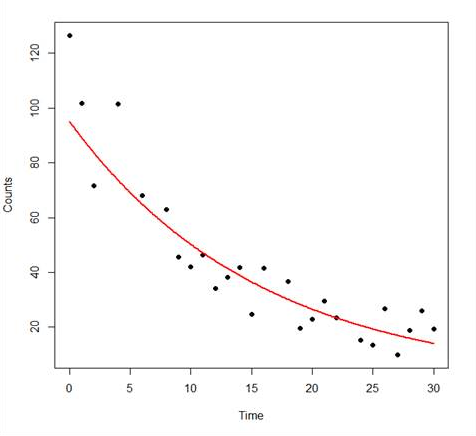
So – we have fitted our exponential model. For our data the fitted exponential model fits the data less well than the quadratic model, but still looks like a good model.

In Part 6 we will look at some basic plotting syntax.

See our full R Tutorial Series and other blog posts regarding R programming

About the Author: David Lillis has taught R to many researchers and statisticians. His company, Sigma Statistics and Research Limited, provides both on-line instruction and face-to-face workshops on R, and coding services in R. David holds a doctorate in applied statistics.

Four Critical Steps in Building Linear Regression Models

While you’re worrying about which predictors to enter, you might be missing issues that have a big impact your analysis. This training will help you achieve more accurate results and a less-frustrating model building experience.

Take Me to The Video!

Tagged as: linear models, Linear Regression, lm, R