count variable

You might already be familiar with the binomial distribution. It describes the scenario where the result of an observation is binary—it can be one of two outcomes. You might label the outcomes as “success” and “failure” (or not!). (more…)

No comments yet

In my last blog post we fitted a generalized linear model to count data using a Poisson error structure.

We found, however, that there was over-dispersion in the data – the variance was larger than the mean in our dependent variable.

(more…)

9 comments

In my last couple of articles (Part 4, Part 5), I demonstrated a logistic regression model with binomial errors on binary data in R’s glm() function.

But one of wonderful things about glm() is that it is so flexible. It can run so much more than logistic regression models.

The flexibility, of course, also means that you have to tell it exactly which model you want to run, and how.

In fact, we can use generalized linear models to model count data as well.

In such data the errors may well be distributed non-normally and the variance usually increases with the mean values.

As with binary data, we use the glm() command, but this time we specify a Poisson error distribution and the logarithm as the link function.

The natural log is the default link function for the Poisson error distribution. It works well for count data as it forces all of the predicted values to be positive.

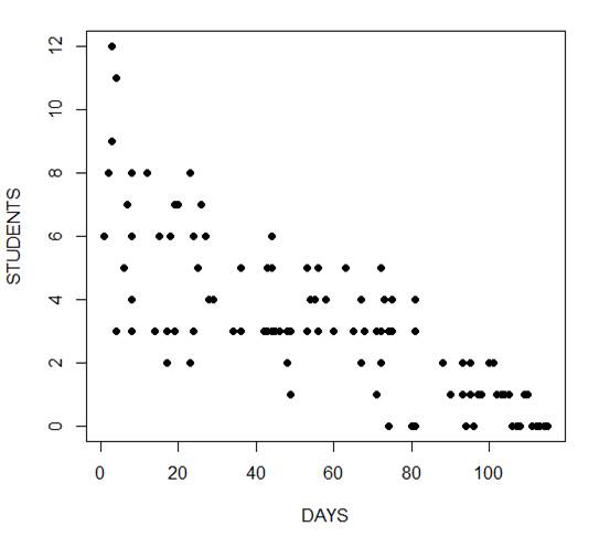
In the following example we fit a generalized linear model to count data using a Poisson error structure. The data set consists of counts of high school students diagnosed with an infectious disease within a period of days from an initial outbreak.

cases <-  
structure(list(Days = c(1L, 2L, 3L, 3L, 4L, 4L, 4L, 6L, 7L, 8L, 
8L, 8L, 8L, 12L, 14L, 15L, 17L, 17L, 17L, 18L, 19L, 19L, 20L, 
23L, 23L, 23L, 24L, 24L, 25L, 26L, 27L, 28L, 29L, 34L, 36L, 36L, 
42L, 42L, 43L, 43L, 44L, 44L, 44L, 44L, 45L, 46L, 48L, 48L, 49L, 
49L, 53L, 53L, 53L, 54L, 55L, 56L, 56L, 58L, 60L, 63L, 65L, 67L, 
67L, 68L, 71L, 71L, 72L, 72L, 72L, 73L, 74L, 74L, 74L, 75L, 75L, 
80L, 81L, 81L, 81L, 81L, 88L, 88L, 90L, 93L, 93L, 94L, 95L, 95L, 
95L, 96L, 96L, 97L, 98L, 100L, 101L, 102L, 103L, 104L, 105L, 
106L, 107L, 108L, 109L, 110L, 111L, 112L, 113L, 114L, 115L), 
    Students = c(6L, 8L, 12L, 9L, 3L, 3L, 11L, 5L, 7L, 3L, 8L, 
    4L, 6L, 8L, 3L, 6L, 3L, 2L, 2L, 6L, 3L, 7L, 7L, 2L, 2L, 8L, 
    3L, 6L, 5L, 7L, 6L, 4L, 4L, 3L, 3L, 5L, 3L, 3L, 3L, 5L, 3L, 
    5L, 6L, 3L, 3L, 3L, 3L, 2L, 3L, 1L, 3L, 3L, 5L, 4L, 4L, 3L, 
    5L, 4L, 3L, 5L, 3L, 4L, 2L, 3L, 3L, 1L, 3L, 2L, 5L, 4L, 3L, 
    0L, 3L, 3L, 4L, 0L, 3L, 3L, 4L, 0L, 2L, 2L, 1L, 1L, 2L, 0L, 
    2L, 1L, 1L, 0L, 0L, 1L, 1L, 2L, 2L, 1L, 1L, 1L, 1L, 0L, 0L, 
    0L, 1L, 1L, 0L, 0L, 0L, 0L, 0L)), .Names = c("Days", "Students"
), class = "data.frame", row.names = c(NA, -109L))

attach(cases)

head(cases) 
    Days Students
1    1      6
2    2      8
3    3     12
4    3      9
5    4      3
6    4      3

The mean and variance are different (actually, the variance is greater). Now we plot the data.

plot(Days, Students, xlab = "DAYS", ylab = "STUDENTS", pch = 16)

Now we fit the glm, specifying the Poisson distribution by including it as the second argument.

model1 <- glm(Students ~ Days, poisson) summary(model1) Call: glm(formula = Students ~ Days, family = poisson) Deviance Residuals: Min 1Q Median 3Q Max -2.00482 -0.85719 -0.09331 0.63969 1.73696 Coefficients: Estimate Std. Error z value Pr(>|z|)    
(Intercept)  1.990235   0.083935   23.71   <2e-16 ***
Days        -0.017463   0.001727  -10.11   <2e-16 ***
---
Signif. codes:  0 ‘***’ 0.001 ‘**’ 0.01 ‘*’ 0.05 ‘.’ 0.1 ‘ ’ 1

(Dispersion parameter for poisson family taken to be 1)

    Null deviance: 215.36  on 108  degrees of freedom
Residual deviance: 101.17  on 107  degrees of freedom
AIC: 393.11

Number of Fisher Scoring iterations: 5

The negative coefficient for Days indicates that as days increase, the mean number of students with the disease is smaller.

This coefficient is highly significant (p < 2e-16).

We also see that the residual deviance is greater than the degrees of freedom, so that we have over-dispersion. This means that there is extra variance not accounted for by the model or by the error structure.

This is a very important model assumption, so in my next article we will re-fit the model using quasi poisson errors.

****

See our full R Tutorial Series and other blog posts regarding R programming.

About the Author: David Lillis has taught R to many researchers and statisticians. His company, Sigma Statistics and Research Limited, provides both on-line instruction and face-to-face workshops on R, and coding services in R. David holds a doctorate in applied statistics.

7 comments