No, degrees of freedom is not “having one foot out the door”!
Definitions are rarely very good at explaining the meaning of something. At least not in statistics. Degrees of freedom: “the number of independent values or quantities which can be assigned to a statistical distribution”.
This is no exception.
Let’s dig into an example to show you what degrees of freedom (df) really are.
We will use linear regression output to explain. Our outcome variable is BMI (body mass index).
Degrees of Freedom with one Parameter Estimate
The starting point for understanding degrees of freedom is the total number of observations in the model. This model has 303 observations, shown in the top right corner. In any given sample, if we haven’t used it yet to calculate anything, every observation is free to vary. So we start with 303 df.
But once we use these observations to estimate a parameter the degrees of freedom change.
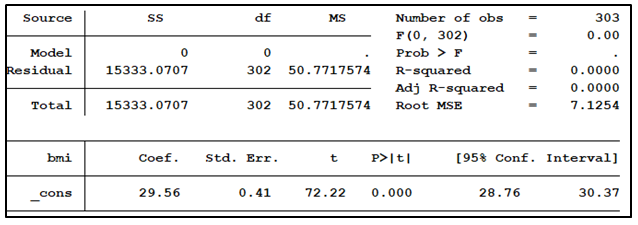
A model run with no predictors, the empty model, provides one estimated parameter value, the intercept (here labeled _cons). The intercept in this model is just the mean of the outcome variable, BMI.
Note that the “Residual” df and the “Total” df are both 302. The empty model has n-1 df, where n = number of observations.
Why does the empty model have n-1 df and not n?
Once we calculate the mean of a series of numbers, we’ve restricted one of the observations. In other words, if I tell you the sample mean and I tell you the value of 302 of the observations, you can tell me with 100% certainty what the value is of the 303rd observation.
It’s like a (really bad) statistical card trick. You’ll always know the value of the last observation in the sample, once you know the mean and the other 302 observations.
The way we think of it statistically: there are no restrictions on the value of those numbers except for one of them.
There are no restrictions as to how the “other” subjects’ BMI can vary. Knowing the mean of BMI, the final subject’s BMI cannot vary.
Here is the mathematical equation:
![]()
In terms of our model above, 302 observations can vary, one cannot. Our empty model has 302 degrees of freedom.
Degrees of Freedom with more Parameter Estimates
What happens when we include a categorical predictor for body frame which has three categories: small, medium and large?
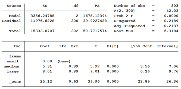
The “Total” number of degrees of freedom remains at n-1, 302. “Model” has been added as a “Source”. Its degrees of freedom is 2. Why?
Because we’ve added two new parameter estimates to the model—the regression coefficients for medium and large. The intercept (_cons) represents the mean value of BMI for the reference group, small frame. Medium frame is estimated to be 5.31 greater than small frame, 30.43. Large frame is estimated to be 8.01 greater than small frame, 33.13.
How do these estimates impact the degrees of freedom?
We use the same mathematical logic here as we did for the empty model.
The Calculations
If we know the mean of BMI for small frame, all but one small frame individual’s observed value can vary.
![]()
If we know the mean of BMI for medium frame, all but one medium frame individual’s observed value can vary.
![]()
If we know the mean of BMI for large frame, all but one large frame individual’s observed value can vary.
![]()
We know the “Total” degrees of freedom equal n-1 as a result of calculating the intercept (mean for small frame individuals). One medium frame observation is no longer free to vary since we know the mean BMI for medium frame observations. The same is true for large frame individuals.
Our model has used a total of 2 degrees of freedom for the additional two mean values estimated. That is why “Model” has 2 df. The residual df represents the number of observations whose BMI can still vary. To calculate the residual’s df we simply subtract the “Model” df from the “Total” df.
Each time we add predictors to the model we add parameters to estimate, so are increasing the “Model” df. If the predictor is continuous, we are adding one df to the “Model” df. If the predictor is categorical, we are adding the number of categories minus one.
In other words, each parameter estimate summarizes the values of the sample observations. With each new summary, one fewer sample observation is free to have any value. So we specify the number of new estimates in the model df. And we specify what’s left over in residual df.
Thank you very much for sharing very important
#observations – #estimated parameters
An example that I’ve used for one parameter (the mean) is to tell the class that I have 3 numbers in my head, the mean of which is 5. Then I ask them to tell me what the 3 numbers are. There is an opportunity for fun as they try to guess the first 2 that, “I have in my head.” Once those 2 are set, someone will get the 3rd and some will wonder how they did it.
Thanks for the clear & intuitive explanation on d.f. Two thumbs up 🙂