 You put a lot of work into preparing and cleaning your data. Running the model is the moment of excitement.
You look at your tables and interpret the results. But first you remember that one or more variables had a few outliers. Did these outliers impact your results? (more…)
There are many steps to analyzing a dataset. One of the first steps is to create tables and graphs of your variables in order to understand what is behind the thousands of numbers on your screen. But the type of table and graph you create depends upon the type of variable you are looking at.
There certainly isn’t much point in running a frequency table for a continuous variable with hundreds of unique observations. Creating a boxplot to look for outliers doesn’t make much sense if the variable is categorical. Creating a histogram for a dummy variable would be senseless as well.
How should you start this process? Should you create a spreadsheet listing all the names of the variables and list what type of variable they are? Should you paste the names into a Word document?
In this free webinar with Stata expert Jeff Meyer, you will discover the code to quickly determine the type of every variable in a dataset. By simply pressing the execute button on a do-file you will observe Stata placing each variable in a group (the macro) based on the type of variable it is.
You will watch, through the use of loops, Stata create the proper table and graph for each type of variable in a matter of minutes and output the data into a pdf file for future viewing. You will also receive the code to recreate and practice what you’ve learned.
**
Title: Improving Your Productivity by Unlocking the Power of Stata’s Macros and Loops
Date: Thurs, May 26, 2016
Time: 1-2 pm EDT
Presenter: Jeff Meyer
This webinar has already taken place. Please sign up below to get access to the video recording.
Jeff Meyer is a statistical consultant with The Analysis Factor, a stats mentor for Statistically Speaking membership, and a workshop instructor. Read more about Jeff here.
In a previous post , Using the Same Sample for Different Models in Stata, we examined how to use the same sample when comparing regression models. Using different samples in our models could lead to erroneous conclusions when interpreting results.
But excluding observations can also result in inaccurate results.
The coefficient for the variable “frequent religious attendance” was negative 58 in model 3 (more…)
In a previous post we explored bounded variables and the difference between truncated and censored. Can we ignore the fact that a variable is bounded and just run our analysis as if the data wasn’t bounded? (more…)
A data set can contain indicator (dummy) variables, categorical variables and/or both. Initially, it all depends upon how the data is coded as to which variable type it is.
For example, a categorical variable like marital status could be coded in the data set as a single variable with 5 values: (more…)
Fortunately there are some really, really smart people who use Stata. Yes I know, there are really, really smart people that use SAS and SPSS as well.
But unlike SAS and SPSS users, Stata users benefit from the contributions made by really, really smart people. How so? Is Stata an “open source” software package?
Technically a commercial software package (software you have to pay for) cannot be open source. Based on that definition Stata, SPSS and SAS are not open source. R is open source.
But, because I have a Stata license (once you have it, it never expires) I think of Stata as being open source. This is because Stata allows members of the Stata community to share their expertise.
There are countless commands written by very, very smart non-Stata employees that are available to all Stata users.
Practically all of these commands, which are free, can be downloaded from the SSC (Statistical Software Components) archive. The SSC archive is maintained by the Boston College Department of Economics. The website is: https://ideas.repec.org/s/boc/bocode.html
There are over three thousand commands available for downloading. Below I have highlighted three of the 185 that I have downloaded.
1. coefplot is a command written by Ben Jann of the Institute of Sociology, University of Bern, Bern, Switzerland. This command allows you to plot results from estimation commands.
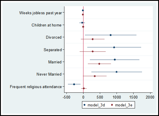
In a recent post on diagnosing missing data, I ran two models comparing the observations that reported income versus the observations that did not report income, models 3d and 3e.
Using the coefplot command I can graphically compare the coefficients and confidence intervals for each independent variable used in the models.
The code and graph are:
coefplot model_3d model_3e, drop(_cons) xline(0)
Including the code xline(0) creates a vertical line at zero which quickly allows me to determine whether a confidence interval spans both positive and negative territory.
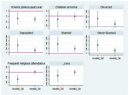
I can also separate the predictor variables into individual graphs:
coefplot model_3d || model_3e, yline(0) bycoefs vertical byopts(yrescale) ylabel(, labsize(vsmall))
2. Nicholas Cox of Durham University and Gary Longton of the Fred Hutchinson Cancer Research Center created the command distinct. This command generates a table with the count of distinct observations for each variable in the data set.
When getting to know a data set, it can be helpful to search for potential indicator, categorical and continuous variables. The distinct command along with its min(#) and max(#) options allows an easy search for variables that fit into these categories.
For example, to create a table of all variables with three to seven distinct observations I use the following code:
distinct, min(3) max(7)
In addition, the command generates the scalar r(ndistinct). In the workshop Managing Data and Optimizing Output in Stata, we used this scalar within a loop to create macros for continuous, categorical and indicator variables.
3. In a data set it is not uncommon to have outliers. There are primarily three options for dealing with outliers. We can keep them as they are, winsorize the observations (change their values), or delete them. Note, winsorizing and deleting observations can introduce statistical bias.
If you choose to winsorize your data I suggest you check out the command winsor2. This was created by Lian Yujun of Sun Yat-Sen University, China. This command incorporates coding from the command winsor created by Nicholas Cox and Judson Caskey.
The command creates a new variable, adding a suffix “_w” to the original variable’s name. The default setting changes observations whose values are less than the 1st percentile to the 1 percentile. Values greater than the 99th percentile are changed to equal the 99th percentile. Example:
winsor2 salary (makes changes at the 1st and 99th percentile for the variable “salary”)
The user has the option to change the values to the percentile of their choice.
winsor2 salary, cuts(0.5 99.5) (makes changes at the 0.5st and 99.5th percentile)
To add these three commands to your Stata software execute the following code and click on the links to download the commands:
findit coefplot
findit distinct
findit winsor2
As shown in the December, 2015 free webinar “Stata’s Bountiful Help Resources”, you can also explore all the add-on commands via Stata’s “Help” menu. Go to “Help” => “SJ and User Written Commands” to explore.
Jeff Meyer is a statistical consultant with The Analysis Factor, a stats mentor for Statistically Speaking membership, and a workshop instructor. Read more about Jeff here.