Incorporating Graphs in Regression Diagnostics with Stata

by Jeff Meyer

You put a lot of work into preparing and cleaning your data. Running the model is the moment of excitement.

You look at your tables and interpret the results. But first you remember that one or more variables had a few outliers. Did these outliers impact your results?

In our upcoming Linear Models in Stata workshop, we will explore ways to find observations that influence the model. This is done in Stata via post-estimation commands. As the name implies, all post-estimation commands are run after running the model (regression, logit, mixed, etc).

One widely-used post-estimation command for linear regression is predict. Predict is very important for detecting outliers and determining their impact on your model.

There are 17 options for using this command. Why so many? One reason is no one measure can tell you everything you need to know about your outliers. Some options are useful for identifying outcome outliers while others identify predictor outliers.

A third group of options are useful for identifying influential observations (since not all outliers are influential).  An observation is considered influential if excluding the observation alters the coefficients of the model .

Studentized residuals are a way to find outliers on the outcome variable.  Values far from 0 and the rest of the residuals indicate outliers on Y.

Leverage is a measurement of outliers on predictor variables. It measures the distance between a case’s X value and the mean of X. Like the residuals, values far from 0 and the rest of the residuals indicate outliers on X.

Cook’s distance is a measure of influence–how much each observation affects the predicted values. It incorporates both outcome (residuals) and predictor (leverage) observations in its calculations, but more importantly tells you how much a case affects the model.

The graph below incorporates measurement for influence, outcome and predictor outliers for a data set comprised of 20 observations with one predictor variable. Each observation’s studentized residual is measured along the y-axis. An observation’s leverage is measured via the x-axis. Each observation’s overall influence on the best fit line is depicted by the size of its circle. There are a few ways to measure an observation’s overall influence. In this example its overall influence is measured by the statistic Cook’s distance.

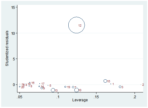
Relying solely on the leverage statistic or the studentized residual will not give you the complete picture of how an observation interacts in influencing the best fit line. Note that observation 12 has a very high studentized residual but a mediocre  leverage value. Observation 10 has a higher overall influence but its residual is quite low and its leverage is moderately high.

Another method for determining the influence an observation has on the model’s coefficients is to run a series of regressions where you emit one observation each time. If your data set has 20 observations you would end up with 20 regression outputs. Using macros and a loop, this process was run on the 20 observations. The slope and y-intercept of each regression were saved in the data set. Those values are graphed below along with the observation’s identifier.

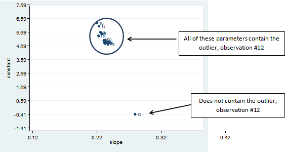
As shown in the graph, if observation 12 is excluded from the linear regression, the slope of the predictor variable increases from approximately 0.22 to 0.28. The intercept decreases from approximately 5.50 to -0.41. If any other single observation is excluded, there are very minor changes to the slope and/or constant. Obviously observation #12 is very influential.

Four Critical Steps in Building Linear Regression Models

While you’re worrying about which predictors to enter, you might be missing issues that have a big impact your analysis. This training will help you achieve more accurate results and a less-frustrating model building experience.

Take Me to The Video!