March 27th, 2013 by Karen Grace-Martin
One of the nice features of SPSS is its ability to keep track of information on the variables themselves.

This includes variable labels, missing data codes, value labels, and variable formats. Spending the time to set up variable information makes data analysis much easier–you don’t have to keep looking up whether males are coded 1 or 0, for example.
And having them all in the variable view window makes things incredibly easy while you’re doing your analysis. But sometimes you need to just print them all out–to create a code book for another analyst or to include in the output you’re sending to a collaborator. Or even just to print them out for yourself for easy reference.
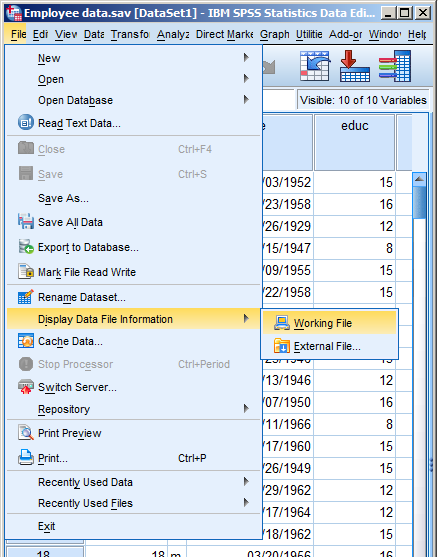
There is a nice little way to get a few tables with a list of all the variable metadata. It’s in the File menu. Simply choose Display Data File Information and Working File.
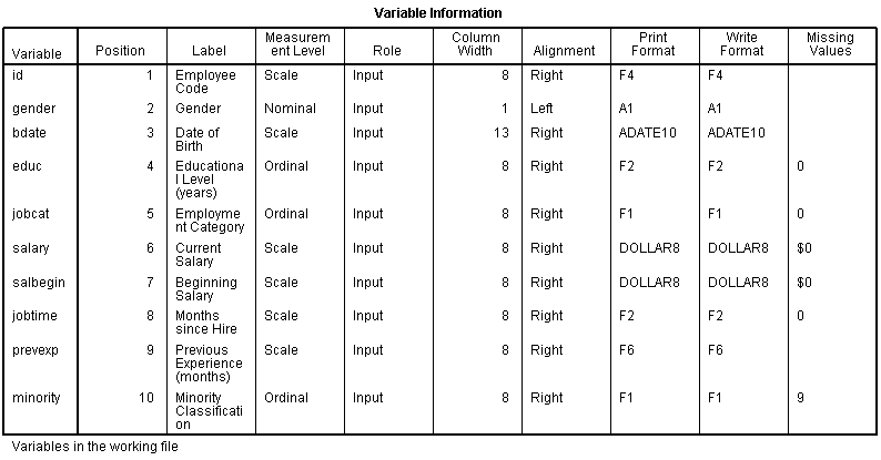
Doing this gives you two tables. The first includes the following information on the variables. I find the information I use the most are the labels and the missing data codes.


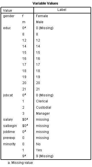
Even more useful, though, is the Value Label table.
It lists out the labels for all the values for each variable.
So you don’t have to remember that Job Category (jobcat) 1 is “Clerical,” 2 is “Custodial,” and 3 is “Managerial.”
It’s all right there.
April 1st, 2011 by Karen Grace-Martin
Here’s a little SPSS tip.
When you create new variables, whether it’s through the Recode, Compute, or some other command, you need to check that it worked the way you think it did.
(As an aside, I hope this goes without saying, but never, never, never, never use Recode into Same Variable. Always Recode into Different Variable so you don’t overwrite your data and then discover you made a mistake. Or worse, not discover. It happens).
And the easiest way to do that is to simply look at the data. (more…)
March 18th, 2011 by guest contributer
by Annette Gerritsen, Ph.D.
In an earlier article I discussed how to do a cross-tabulation in SPSS. But what if you do not have a data set with the values of the two variables of interest?
For example, if you do a critical appraisal of a published study and only have proportions and denominators.
In this article it will be demonstrated how SPSS can come up with a cross table and do a Chi-square test in both situations. And you will see that the results are exactly the same.
‘Normal’ dataset
If you want to test if there is an association between two nominal variables, you do a Chi-square test.
In SPSS you just indicate that one variable (the independent one) should come in the row, (more…)
March 11th, 2011 by Karen Grace-Martin
SPSS offers two choices under the recode command: Into Same Variable and Into Different Variables.
The command Into Same Variable replaces existing data with new values, but the command Into Different Variables adds a new variable to the data set.
In almost every situation, you want to use Into Different Variables. Recoding Into Same Variables replaces the values in the existing variable.
So if you notice a mistake after you’ve recoded, you can’t fix it.
But you may not even notice the mistake, because you can’t even test it.
And that’s just dangerous. (more…)
October 21st, 2010 by Karen Grace-Martin
One of the places that SPSS syntax excels at efficiency is when you’re creating new variables. This is especially true when you’re creating a LOT of new variables, but even one or two can be quicker if you write the syntax code instead of menus.
And just as importantly, you’ll have documentation for exactly how you created them. (You think you’ll remember now, but 75 new variables later, you’ll thank me).
So once you create a new variable, you should of course immediately assign a Variable Label, and if appropriate, Value Labels and Missing Data Codes using Syntax.
Another thing that helps keep your new variable clean and interpretable is to assign the format. The default format is F8.2, which indicates a numerical value
You could go into the Variable View screen and manually change the Width and Decimals columns, which indicate how many characters go before and after (for numeric variables) the decimal point.
But why do all that when you can just use a single command to define multiple variables?
The syntax command is FORMATS. Here is the command for some common formats:
FORMATS NumVar1 NumVar2 (F5.0)
/NumVar3 (F6.1)
/StringVar1 (A15).
You can see the FORMATS command is followed by the variable names, then the format in parentheses.
Numeric variables NumVar1 and Numvar2 will both get the same format: with 5 digits, and nothing after the decimal.
Numeric variable NumVar3 will have 6 digits total, with one after the decimal.
And string variable (i.e. its value contain letters) StringVar1 is 15 characters wide.
This will get you started, but you can get all the specifics in the FORMATS section of the Command Syntax Reference, which is included in the SPSS help.
[Note: Edited explanation of F6.1 to be 6 digits total, not 6 digits before the decimal).
September 3rd, 2010 by guest contributer
by Annette Gerritsen, Ph.D.
Cross-tabulation in cohort studies
Assume you have just done a cohort study. How do you actually do the cross-tabulation to calculate the cumulative incidence in both groups?
Best is to always put the outcome variable (disease yes/no) in the columns and the exposure variable in the rows. In other words, put the dependent variable–the one that describes the problem under study–in the columns. And put the independent variable–the factor assumed to cause the problem–in the rows.
Let’s take as example a cohort study used to see whether there is a causal relationship between the use of a certain water source and the incidence of diarrhea among children under five in a village with different water sources. In this case, the variable diarrhea (yes/no) should be in the columns. The variable water source (suspected/other) should be in the rows.
SPSS will put the lowest value of the variable in the first column or row. So in order to get those with diarrhea in the first column you should label ‘diarrhea’ as 1 and ‘no diarrhea’ as 2. The same is true for the exposure variable: label the ‘suspected water source’ as 1 and the ‘other water source’ as 2.
You will then be able to calculate the cumulative incidence (risk of developing the disease) among those with the exposure: a / (a + b) and among those without the exposure: c / (c + d).
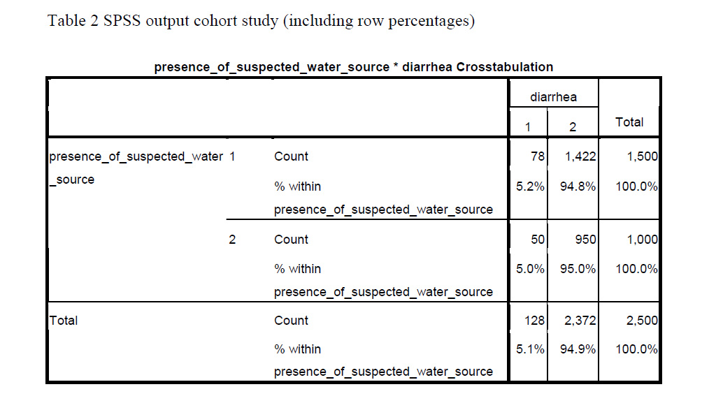
In the case of the diarrhea study (Table 1), you could calculate the cumulative incidence of diarrhea among those exposed to the suspected water source, which would be (78 / 1,500 =) 5.2%.
You can also do this for those exposed to other water sources, which would be (50 / 1,000 =) 5.0%.

SPSS can give you these percentages immediately (in cell ‘a’ and ‘c’ respectively), when you ask to display row percentages in the Cells option (Table 2).

Cross-tabulation in Case-Control Studies
When you have used a case-control design for the diarrhea study, the actual cross-tabulation is quite similar, only “presence of diarrhea yes/no”, is now changed into “cases” and “controls.
Label the cases as 1, and the controls as 2. Be aware that row percentages have no meaning in terms of occurrence of disease in case-control studies. This is because in case-control studies the researcher determines how many patients and how many controls are included.
The ratio between the number of patients and controls (e.g. 2 : 1 or 4 : 1) influences the row percentages. So in a case-control study, the cumulative incidence cannot be calculated.
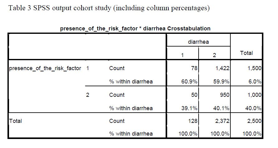
When having conducted a case-control study, you can ask to display column percentages. That gives you the proportion of those exposed to the suspected water source among the cases (in cell ‘a’) and among the controls (in cell ‘b’).
Table 3 gives the SPSS output for the same diarrhea study assuming that it had a case-control design. Using the data provided, (78 / 128 =) 60.9% of the cases were exposed to the suspected water source, while this was (1,422 / 2,372 =) 59.9% of the controls (asked for column percentages).

Another article will be devoted to measures of association: How do you actually compare cumulative incidence rates in cohort studies? And what measure of association can be used in case-control studies?
About the Author: With expertise in epidemiology, biostatistics and quantitative research projects, Annette Gerritsen, Ph.D. provides services to her clients focussing on the methodological soundness of each phase of an epidemiological study to ensure getting valid answers to the proposed research questions. She is the founder of Epi Result.

