I recently gave a free webinar on Principal Component Analysis. We had almost 300 researchers attend and didn’t get through all the questions. This is part of a series of answers to those questions.
If you missed it, you can get the webinar recording here.
Question: Can we use PCA for reducing both predictors and response variables?
In fact, there were a few related but separate questions about using and interpreting the resulting component scores, so I’ll answer them together here.
How could you use the component scores?
A lot of times PCAs are used for further analysis — say, regression. How can we interpret the results of regression?
Let’s say I would like to interpret my regression results in terms of original data, but they are hiding under PCAs. What is the best interpretation that we can do in this case?
Answer:
So yes, the point of PCA is to reduce variables — create an index score variable that is an optimally weighted combination of a group of correlated variables.
And yes, you can use this index variable as either a predictor or response variable.
It is often used as a solution for multicollinearity among predictor variables in a regression model. Rather than include multiple correlated predictors, none of which is significant, if you can combine them using PCA, then use that.
It’s also used as a solution to avoid inflated familywise Type I error caused by running the same analysis on multiple correlated outcome variables. Combine the correlated outcomes using PCA, then use that as the single outcome variable. (This is, incidentally, what MANOVA does).
In both cases, you can no longer interpret the individual variables.
You may want to, but you can’t. (more…)
One of the many confusing issues in statistics is the confusion between Principal Component Analysis (PCA) and Factor Analysis (FA).
They are very similar in many ways, so it’s not hard to see why they’re so often confused. They appear to be different varieties of the same analysis rather than two different methods. Yet there is a fundamental difference between them that has huge effects on how to use them.
(Like donkeys and zebras. They seem to differ only by color until you try to ride one).
Both are data reduction techniques—they allow you to capture the variance in variables in a smaller set.
Both are usually run in stat software using the same procedure, and the output looks pretty much the same.
The steps you take to run them are the same—extraction, interpretation, rotation, choosing the number of factors or components.
Despite all these similarities, there is a fundamental difference between them: PCA is a linear combination of variables; Factor Analysis is a measurement model of a latent variable.
Principal Component Analysis
PCA’s approach to data reduction is to create one or more index variables from a larger set of measured variables. It does this using a linear combination (basically a weighted average) of a set of variables. The created index variables are called components.
The whole point of the PCA is to figure out how to do this in an optimal way: the optimal number of components, the optimal choice of measured variables for each component, and the optimal weights.
The picture below shows what a PCA is doing to combine 4 measured (Y) variables into a single component, C. You can see from the direction of the arrows that the Y variables contribute to the component variable. The weights allow this combination to emphasize some Y variables more than others.
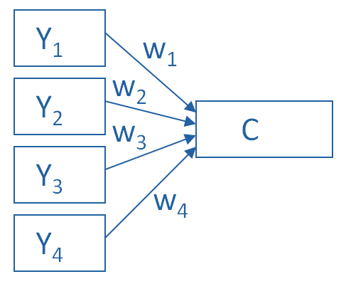
This model can be set up as a simple equation:
C = w1(Y1) + w2(Y2) + w3(Y3) + w4(Y4)
Factor Analysis
A Factor Analysis approaches data reduction in a fundamentally different way. It is a model of the measurement of a latent variable. This latent variable cannot be directly measured with a single variable (think: intelligence, social anxiety, soil health). Instead, it is seen through the relationships it causes in a set of Y variables.
For example, we may not be able to directly measure social anxiety. But we can measure whether social anxiety is high or low with a set of variables like “I am uncomfortable in large groups” and “I get nervous talking with strangers.” People with high social anxiety will give similar high responses to these variables because of their high social anxiety. Likewise, people with low social anxiety will give similar low responses to these variables because of their low social anxiety.
The measurement model for a simple, one-factor model looks like the diagram below. It’s counter intuitive, but F, the latent Factor, is causing the responses on the four measured Y variables. So the arrows go in the opposite direction from PCA. Just like in PCA, the relationships between F and each Y are weighted, and the factor analysis is figuring out the optimal weights.
In this model we have is a set of error terms. These are designated by the u’s. This is the variance in each Y that is unexplained by the factor.
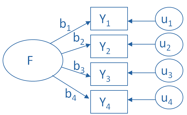
You can literally interpret this model as a set of regression equations:
Y1 = b1*F + u1
Y2 = b2*F + u2
Y3 = b3*F + u3
Y4 = b4*F + u4
As you can probably guess, this fundamental difference has many, many implications. These are important to understand if you’re ever deciding which approach to use in a specific situation.
Go to the next article or see the full series on Easy-to-Confuse Statistical Concepts
Here’s a question I get pretty often: In Principal Component Analysis, can loadings be negative and positive?
Answer: Yes.
Recall that in PCA, we are creating one index variable (or a few) from a set of variables. You can think of this index variable as a weighted average of the original variables.
The loadings are the correlations between the variables and the component. We compute the weights in the weighted average from these loadings.
The goal of the PCA is to come up with optimal weights. “Optimal” means we’re capturing as much information in the original variables as possible, based on the correlations among those variables.
So if all the variables in a component are positively correlated with each other, all the loadings will be positive.
But if there are some negative correlations among the variables, some of the loadings will be negative too.
An Example of Negative Loadings in Principal Component Analysis
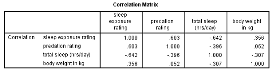
Here’s a simple example that we used in our Principal Component Analysis webinar. We want to combine four variables about mammal species into a single component.
The variables are weight, a predation rating, amount of exposure while sleeping, and the total number of hours an animal sleeps each day.
If you look at the correlation matrix, total hours of sleep correlates negatively with the other 3 variables. Those other three are all positively correlated.
It makes sense — species that sleep more tend to be smaller, less exposed while sleeping, and less prone to predation. Species that are high on these three variables must not be able to afford much sleep.
Think bats vs. zebras.
Likewise, the PCA with one component has positive loadings for three of the variables and a negative loading for hours of sleep.
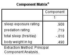
Species with a high component score will be those with high weight, high predation rating, high sleep exposure, and low hours of sleep.
It’s that time of year: flu season.
Let’s imagine you have been asked to determine the factors that will help a hospital determine the length of stay in the intensive care unit (ICU) once a patient is admitted.
The hospital tells you that once the patient is admitted to the ICU, he or she has a day count of one. As soon as they spend 24 hours plus 1 minute, they have stayed an additional day.
Clearly this is count data. There are no fractions, only whole numbers.
To help us explore this analysis, let’s look at real data from the State of Illinois. We know the patients’ ages, gender, race and type of hospital (state vs. private).
A partial frequency distribution looks like this: (more…)
In a previous article, we discussed how incidence rate ratios calculated in a Poisson regression can be determined from a two-way table of categorical variables.
Statistical software can also calculate the expected (aka predicted) count for each group. Below is the actual and expected count of the number of boys and girls participating and not participating in organized sports.
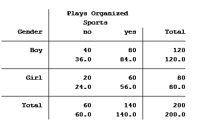
The value in the top of each cell is the actual count (40 boys do not play organized sports) and the bottom value is the expected/predicted count (36 boys are predicted to not play organized sports).
The Poisson model that we ran in the previous article generated the following table: (more…)
The coefficients of count model regression tables are shown in either logged form or as incidence rate ratios. Trying to explain the coefficients in logged form can be a difficult process.
Incidence rate ratios are much easier to explain. You probably didn’t realize you’ve seen incidence rate ratios before, expressed differently.
Let’s look at an example.
A school district was interested in how many children in their sixth grade classes played on organized sports teams. So they did a count and also noted the gender of the child. The results were put into a table: (more…)