 Centering variables is common practice in some areas, and rarely seen in others. That being the case, it isn’t always clear what are the reasons for centering variables.
 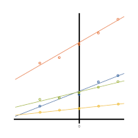 Is it only a matter of preference, or does centering variables help with analysis and interpretation? (more…)
Stage 2
Member Training: Centering
November 30th, 2022 by TAF Support
What is a Completely Randomized Design?
November 8th, 2022 by Kim Love
The most basic experimental design is the completely randomized design. It is simple and straightforward when plenty of unrelated subjects are available for an experiment. It’s so simple, it almost seems obvious. But there are important principles in this simple design that are important for tackling more complex experimental designs.
Let’s take a look.
How It Works
The basic idea of any experiment is to learn how different conditions or versions of a treatment affect an outcome. To do this, you assign subjects to different treatment groups. You then run the experiment and record the results for each subject.
Afterward, you use statistical methods to determine whether the different treatment groups have different outcomes.
Key principles for any experimental design are randomization, replication, and reduction of variance. Randomization means assigning the subjects to the different groups in a random way.
Replication means ensuring there are multiple subjects in each group.
Reduction of variance refers to removing or accounting for systematic differences among subjects. Completely randomized designs address the first two principles in a simple way.
To execute a completely randomized design, first determine how many versions of the treatment there are. Next determine how many subjects are available. Divide the number of subjects by the number of treatments to get the number of subjects in each group.
The final design step is to randomly assign individual subjects to fill the spots in each group.
Example
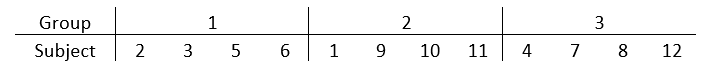
Suppose you are running an experiment. You want to compare three training regimens that may affect the time it takes to run one mile. You also have 12 human subjects who are willing to participate in the experiment. Because you have three training regimens, you will have 12/3 = 4 subjects in each group.
Statistical software (or even Excel) can do the actual assignment. You only need to start by numbering the subjects from 1 to 12 in any way that is convenient. The following table shows one possible random assignment of 12 subjects to three groups.
It’s okay if the number of replicates in each group isn’t exactly the same. Make them as even as possible and assign more to groups that are more interesting to you. Modern statistical software has no trouble adjusting for different sample sizes.
When there is more than one treatment variable, not much changes. Use the combination of treatments when performing random assignment.
For example, say that you add a diet treatment with two conditions in addition to the training. Combined with the three versions of training, there are six possible treatment groups. Assign the subjects in the exact way already described, but with six groups instead of three.
Do not skip randomization! Randomization is the only way to ensure your groups are similar except for the treatment. This is important to ensuring you can attribute group differences to the treatment.
When This Design DOESN’T Work
The completely randomized design is excellent when plenty of unrelated subjects are available to sample. But some situations call for more advanced designs.
This design doesn’t address the third principle of experimental design, reduction of variance.
Sure, you may be able to address this by adding covariates to the analysis. These are variables that are not experimentally assigned but you can measure them. But if reduction of variance is important, other designs do this better.
If some of the subjects are related to each other or a single subject is exposed to multiple conditions of a treatment, you’re going to need another design.
Sometimes it is important to measure outcomes more than once during experimental treatment. For example, you might want to know how quickly the subjects make progress in their training. Again, any repeated measures of outcomes constitute a more complicated design.
Strengths of the Completely Randomized Design
When it works, it has many strengths.
It’s not only easy to create, it’s straightforward to analyze. The results are relatively easy to explain to a non-statistical audience.
Finally, familiarity with this design will help you recognize when it isn’t appropriate. Understanding the ways in which it is not appropriate can help you choose a more advanced design.
The Difference Between R-squared and Adjusted R-squared
August 22nd, 2022 by Karen Grace-Martin
When is it important to use adjusted R-squared instead of R-squared?
R², the Coefficient of Determination, is one of the most useful and intuitive statistics we have in linear regression.
It tells you how well the model predicts the outcome and has some nice properties. But it also has one big drawback.
Member Training: Assumptions of Linear Models
June 30th, 2022 by TAF Support
What are the assumptions of linear models? If you compare two lists of assumptions, most of the time they’re not the same.
(more…)
Member Training: Analyzing Pre-Post Data
May 31st, 2022 by TAF Support
Recommendations on how to analyze pre-post data can vary. Typical recommendations include regression analysis or matched pairs analysis for within subject studies and analysis of covariance (ANCOVA) or linear mixed effects model analysis for within and between subject studies.
(more…)
Three Principles of Experimental Designs
April 19th, 2022 by Kim Love
If you analyze non-experimental data, is it helpful to understand experimental design principles?
Yes, absolutely! Understanding experimental design can help you recognize the questions you can and can’t answer with the data. It will also help you identify possible sources of bias that can lead to undesirable results. Finally, it will help you provide recommendations to make future studies more efficient. (more…)