Measurement Invariance and Multiple Group Analysis

Creating a quality scale for a latent construct (a variable that cannot be directly measured with one variable) takes many steps. Structural Equation Modeling is set up well for this task.

One important step in creating scales is making sure the scale measures the latent construct equally well and the same way for different groups of individuals.

For example, does your scale measure anxiety equally well for adults, adolescents, and children? (Maybe fear of the dark is important for the measure for children, but not adults). Or does your scale measure assertiveness the same way for men and women?

When a scale measures a construct the same for different groups, this is called measurement invariance. Measurement invariance is something you can’t assume. You have to test it.

There are two methods for testing for measurement invariance: multiple group analysis, and a simpler approach known as CFA with covariates. In this article we will focus on measurement invariance using multiple group analysis.

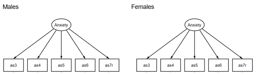
Multiple group analysis allows us to compare loadings, intercepts and error terms in the groups’ measurement models. To have strong invariance, we need to show equal loadings of variables onto the latent variable and equal intercepts between groups. Conceptually, the comparison between groups is shown below.

How can we determine the construct is measured consistently across groups?

There is a multi-step process .The required steps are in this order:

Step 1:

Rerun the Exploratory Factor Analysis (EFA) model separately for both groups.
If different indicator variables load onto the constructs across groups, we go no further. The construct is inconsistent across groups. This is known as testing for dimensional invariance.

Step 2:

After Step 1, we’ve established that for both groups, we use the same indicator variables to measure the construct. Next we establish that their loadings and intercepts are similar.

Run a single model in which the two groups each have their own measurement model. The indicators will be the same for each group, but you allow the software to estimate the loadings and intercepts uniquely for each group.
The loadings and intercepts will rarely be the same for both groups. But the question is, are they similar enough to be considered statistically the same?

In the table below are the estimated loadings and intercepts for the male and female measurement models. This is called the configural model:

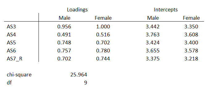
They’re not identical, but are they close enough?

Now refit the model with the two groups. But this time, force the factor loadings to be equal across groups. Allow the intercepts to be unequal. This model is called the metric model.

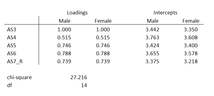
You can see that all the loadings are the same between males and females, but the intercepts are different.
But the chi-square model fit statistics are different. If the difference in chi-square between the two models is small, the factor loadings are considered equivalent across models.

The change in chi-square above is 1.252, 5 degrees of freedom, with a large p-value of 0.81.
Why are the loadings equivalent if the change in chi-square is insignificant? This concept is similar to running a likelihood ratio test for nested models.

The configural model will have n estimated parameters more than the metric model where n is the number of indicators in the latent construct. The models are considered nested because one model has additional parameters.

If there is no real difference in model fit between the configural and metric models we will choose the model that is more parsimonious. The metric model is more parsimonious because we are estimating one set of loadings for both groups’ construct. The configural model estimates different loadings for each group.

If the chi-square difference between the configural and metric models is insignificant we then move on to step 3.

Step 3:

Fit the model with the factor loadings and intercepts equal across all groups. This is known as the scalar model.

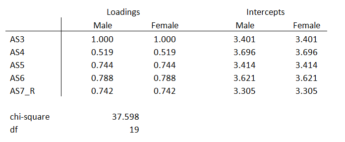
Once again, take the difference between the metric and the scalar chi square model estimates. If the chi-square difference between the metric and scalar models is insignificant, we have group invariance. The change in chi-square above is 10.382, 5 degrees of freedom, p-value 0.065.

If we have group invariance, we know the construct is being measured the same across groups. We can then compare the differences between groups in a path analysis.

A Graphical Example

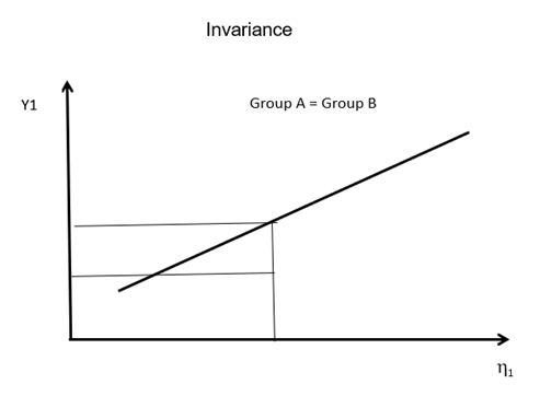
Group invariance is shown graphically below. The graph focuses on only one indicator, Y1. This relationship must hold true for all indicators in order to have group invariance. This is the same graph used to show measurement invariance for the MIMIC model.

The y-axis is the scale of Y1. The x-axis is the scale of the latent construct, n1.

The diagonal line is the relationship between Y1 and n1. This relationship is expressed as the factor loading (the slope). As Y1 increases, the score of the latent construct increases.
When the slope and the intercept are consistent for all matching indicators across groups, we have group invariance.

If the slopes and intercepts are not consistent, as shown below, we have group non-invariance.

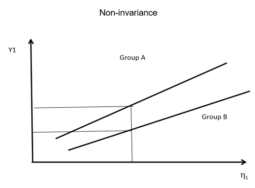
In these situations, we cannot compare the construct between groups.

3 Overlooked Strengths of Structural Equation Modeling

Confirmatory factor analysis (CFA) and path models make up two core building blocks of SEM. Learn how these help you understand how SEM is used.

Sign Up for the Free Webinar!