In our last article, we learned about model fit in Generalized Linear Models on binary data using the glm() command. We continue with the same glm on the mtcars data set (regressing the vs variable on the weight and engine displacement).
Now we want to plot our model, along with the observed data.
Although we ran a model with multiple predictors, it can help interpretation to plot the predicted probability that vs=1 against each predictor separately. So first we fit a glm for only one of our predictors, wt.
model_weight <- glm(vs ~ wt,data=mtcars,family=binomial)
summary(model_weight)
Call:
glm(formula = vs ~ wt, family = binomial, data = mtcars)
Deviance Residuals:
    Min       1Q   Median       3Q      Max
-1.9003  -0.7641  -0.1559   0.7223   1.5736
Coefficients:
            Estimate Std. Error z value Pr(>|z|)
(Intercept)   5.7147     2.3014   2.483  0.01302 *
wt           -1.9105     0.7279  -2.625  0.00867 **
---
Signif. codes:  0 ‘***’ 0.001 ‘**’ 0.01 ‘*’ 0.05 ‘.’ 0.1 ‘ ’ 1
(Dispersion parameter for binomial family taken to be 1)
Null deviance: 43.860  on 31  degrees of freedom
Residual deviance: 31.367  on 30  degrees of freedom
AIC: 35.367
Number of Fisher Scoring iterations: 5
To plot our model we need a range of values of weight for which to produce fitted values. This range of values we can establish from the actual range of values of wt.
range(mtcars$wt)

[1] 1.513 5.424
A range of wt values between 0 and 6 would be ideal. So we create a sequence of values between 0 and 6 in increments of 0.01. Joining such a large number of closely spaced points will give a smooth appearance to our model.
xweight <- seq(0, 6, 0.01)
Now we use the predict() function to create the model for all of the values of xweight.
yweight <- predict(model_weight, list(wt = xweight),type="response")
Now we plot.
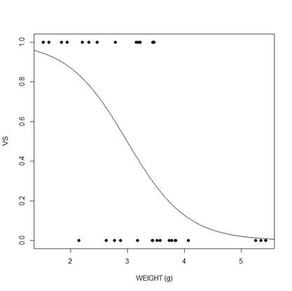
plot(mtcars$wt, mtcars$vs, pch = 16, xlab = "WEIGHT (g)", ylab = "VS")
lines(xweight, yweight)
We can do the same for displacement.
model_disp <- glm(vs ~ disp, family = binomial, data = mtcars)
summary(model_disp)
Call:
glm(formula = vs ~ disp, family = binomial, data = mtcars)
Deviance Residuals:
    Min       1Q   Median       3Q      Max
-1.8621  -0.4143  -0.0872   0.5694   1.8157
Coefficients:
             Estimate Std. Error z value Pr(>|z|)
(Intercept)  4.137827   1.389354   2.978  0.00290 **
disp        -0.021600   0.007131  -3.029  0.00245 **
---
Signif. codes:  0 ‘***’ 0.001 ‘**’ 0.01 ‘*’ 0.05 ‘.’ 0.1 ‘ ’ 1
(Dispersion parameter for binomial family taken to be 1)
Null deviance: 43.860  on 31  degrees of freedom
Residual deviance: 22.696  on 30  degrees of freedom
AIC: 26.696
Number of Fisher Scoring iterations: 6
range(mtcars$disp)
[1]  71.1 472.0
xdisp <- seq(50, 500, 0.01)
ydisp <- predict(model_disp, list(disp = xdisp),type="response")
plot(mtcars$disp, mtcars$vs, pch = 16, xlab = "DISPLACEMENT (cubic inches)", ylab = "VS")
lines(xdisp, ydisp)
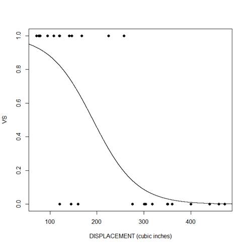
We can see that for both predictors, there is a negative relationship between the probability that vs=1 and the predictor variable. As the predictor increases, the probability decreases.
That wasn’t so hard! In our next article, we will look at other applications of the glm() function.
About the Author: David Lillis has taught R to many researchers and statisticians. His company, Sigma Statistics and Research Limited, provides both on-line instruction and face-to-face workshops on R, and coding services in R. David holds a doctorate in applied statistics.
See our full R Tutorial Series and other blog posts regarding R programming.
I m sorry for the previous post.(in french)
I would like to know how to interprete and present the output of a Glm on R
thantk you
Hi David,
Thank you for your time and help to put this website together, it’s really helpful! I’m trying to plot something slightly different and I was wondering if you could help me find the right line of code.
I want to plot a generalised linear model with only one predictor variable, but I also want to add the intervals of confidence to the fitted line. Is such a thing possible to do?
Thanks in advance!
I’m Veronica again. I forgot to mention I used negative binomial distribution for my model.
Hello together,
how to deal with the plot, if the probabilities are obtained with triangular distribution.
Thank for your response
Thank you so much for putting this on your website. It has been tremendously helpful!
Thanks for this very useful, but I got a bit confused I have followed this from Part 1 then I noticed the coefficient of weight in this part three is now negative compared to part 2 is it because in part 2 it is 2 independent variables but still it wouldnt change that much.
I am trying plotting of my models and residuals. but my problem is that i have one dependent variable which is numeric and other significant independent variable are categorical variables. how do i plot this?I am use glm.poison to estimate my counting data model.
Hello,
Please help me with below situation.
For multivariate logistics regression how to plot the graph. Here all the examples are between one dependent and one independent variable. I am unable to plot the graph if there are multiple independent variable.
Thank You
Anupam
Hello, thx for the tutorial. I have a problem with my glm, my dates are continuos and negatives, so I used gaussian distribution, but when I plot it the line doesn´t have sense, ’cause appear like two lines, likes this: _____________ from xweight to and weight (for example).
Thanks!
Best regards!!
hey,
I use glm.nb to estimate my counting model, I extract my fitted.values, but when I want to add this fitted values to my original data, I get: “The lengths of the variables differ”, and when I look in my regression i fund that “4366 observations deleted due to missingnes” and I have 5156 observation,
so how I can add the fitted values to mydata?
cordially
Coefficients in a polynomial glm with family binomial and fit a curve to scatter plot
I have used glm with quasibinomial error to look at the effect of productivity and initial density on proportion of insect emigration.
The productivity did not have any effect and I reached to the following final model:
Model5=glm(y~NF+NF2,quasibinomial)
I need to use this model to fit a curve to my scatter plot to show the quadratic effect of initial density on proportion emigrating. What I read was to use the coefficients from the summary table of this model to make the line:
Coefficients:
Estimate Std. Error t value Pr(>|t|)
(Intercept) 1.47047 0.89089 1.651 0.1104
NF -0.87076 0.41867 -2.080 0.0472 *
NF2 0.06405 0.03056 2.096 0.0456 *
I looked at this example you provided in your page and I was wondering how you can plot curve on scatter plot when you have quadratic effect of the same variable (in my case NF2)?When i try to follow what you did for your example I keep getting the following error:
x y<- predict(model5, list(NF=x),type="response")
Error in model.frame.default(Terms, newdata, na.action = na.action, xlev = object$xlevels) :
variable lengths differ (found for 'NF2')
When I use the coefficients and make this equation ProEmig=1.470466- 0.870759NF+0.064054NF2 it does not fit into my data correctly.
NF<- seq(0, 12, by=0.1)
lines( NF, 1.470466- 0.870759NF + 0.064054NF^2)
plot(NF,ProEmig,main="Polynomial Model",xlab="NF",ylab="ProEmig")
I read something about back transforming the coefficients but I am not sure if the reason I am not getting the correct line is because I need to the transformation and if yes how I am going to do that?
I am really confused to make the line and I appreciate any help and suggestion.
Thank you.
Dear David,
Yhanks for your support; i need a solution: If I want consider two variabiles in my model, how can i make the plot?
I have
dipendent : happiness
predictors : friends , income
Thanks
BEST Regards
Just had the same doubt as Andrea. Is such a graph possible?
Hi I was wondering the same, any answer?
Hi Andrea
I was wondering if you had already figured it out how to plot this double-fixed models