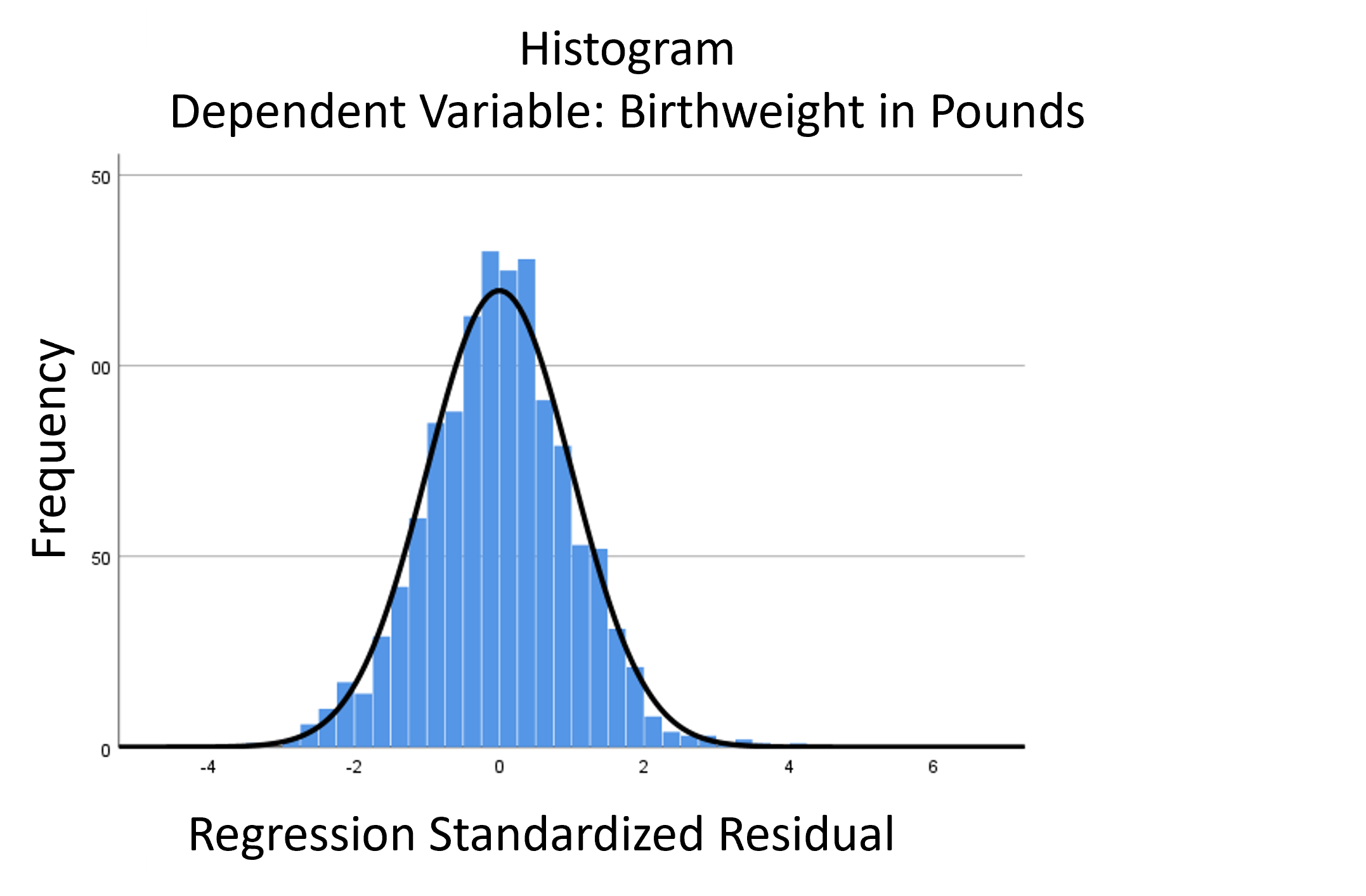
A normal probability plot is extremely useful for checking normality assumptions. It’s more precise than a histogram, which can’t pick up subtle deviations. And yet it doesn’t suffer from too much power from large samples with tiny departures from normality or too little power from small samples with large departures from normality, as do tests like Shaprio-Wilkes.
The biggest problem with a normal probability plot is that it’s hard to read, especially if you’re not used to them. So let’s take a moment and walk through exactly how they work and what they tell you.
There are two versions of normal probability plot: Q-Q and P-P. I’ll start with the Q-Q. (more…)
The linear model normality assumption, along with constant variance assumption, is quite robust to departures. That means that even if the  assumptions aren’t met perfectly, the resulting p-values and confidence intervals will still be reasonable estimates.
This is great because it gives you a bit of leeway to run linear models, which are intuitive and (relatively) straightforward. This is true for both linear regression and ANOVA.
You do need to check the assumptions anyway, though. You can’t just claim robustness and not check. Why? Because some departures are so far off that the p-values and confidence intervals become inaccurate. And in many cases there are remedial measures you can take to turn non-normal residuals into normal ones.
But sometimes you can’t.
Sometimes it’s because the dependent variable just isn’t appropriate for a linear model. The (more…)
I recently received a great question in a comment about whether the assumptions of normality, constant variance, and independence in linear models are about the errors, εi, or the response variable, Yi.
The asker had a situation where Y, the response, was not normally distributed, but the residuals were.
Quick Answer: It’s just the errors.
In fact, if you look at any (good) statistics textbook on linear models, you’ll see below the model, stating the assumptions: (more…)
The normal distribution is so ubiquitous in statistics that those of us who use a lot of statistics tend to forget it’s not always so common in actual data.
And since the normal distribution is continuous, many people describe all numerical variables as continuous. I get it: I’m guilty of using those terms interchangeably, too, but they’re not exactly the same.
Numerical variables can be either continuous or discrete.
The difference? Continuous variables can take any number within a range. Discrete variables can only take on specific values. For numeric discrete data, these are often, but don’t have to be, whole numbers*.
Count variables, as the name implies, are frequencies of some event or state. Number of arrests, fish (more…)
The assumptions of normality and constant variance in a linear model (both OLS regression and ANOVA) are quite robust to departures. That means that even if the assumptions aren’t met perfectly, the resulting p-values will still be reasonable estimates.
But you need to check the assumptions anyway, because some departures are so far off that the p-values become inaccurate. And in many cases there are remedial measures you can take to turn non-normal residuals into normal ones.
But sometimes you can’t.
Sometimes it’s because the dependent variable just isn’t appropriate for a linear model. The (more…)
Here’s a little reminder for those of you checking assumptions in regression and ANOVA:
The assumptions of normality and homogeneity of variance for linear models are not about Y, the dependent variable. (If you think I’m either stupid, crazy, or just plain nit-picking, read on. This distinction really is important). (more…)