The normal distribution is so ubiquitous in statistics that those of us who use a lot of statistics tend to forget it’s not always so common in actual data.
And since the normal distribution is continuous, many people describe all numerical variables as continuous. I get it: I’m guilty of using those terms interchangeably, too, but they’re not exactly the same.
Numerical variables can be either continuous or discrete.
The difference? Continuous variables can take any number within a range. Discrete variables can only take on specific values. For numeric discrete data, these are often, but don’t have to be, whole numbers*.
Count variables, as the name implies, are frequencies of some event or state. Number of arrests, fish in a trap, wetlands in a forest are all counts. They’re numerical and discrete, not continuous.
Not only are they discrete, they can’t be negative. You can have 0 or 4 fish in the trap, but not -8.
This point is extremely important for statistical modeling. Count variables have a lower bound at 0 but no upper bound.
A normal distribution, on the other hand, has no bounds. Theoretically, any value from -∞ to ∞ is possible in a normal distribution.
Count variables tend to follow distributions like the Poisson (or negative binomial, which can be derived as an extension of the Poisson). Both are discrete and bounded at 0.
Unlike normal distributions, which are always symmetric, the basic shape of a Poisson distribution changes.
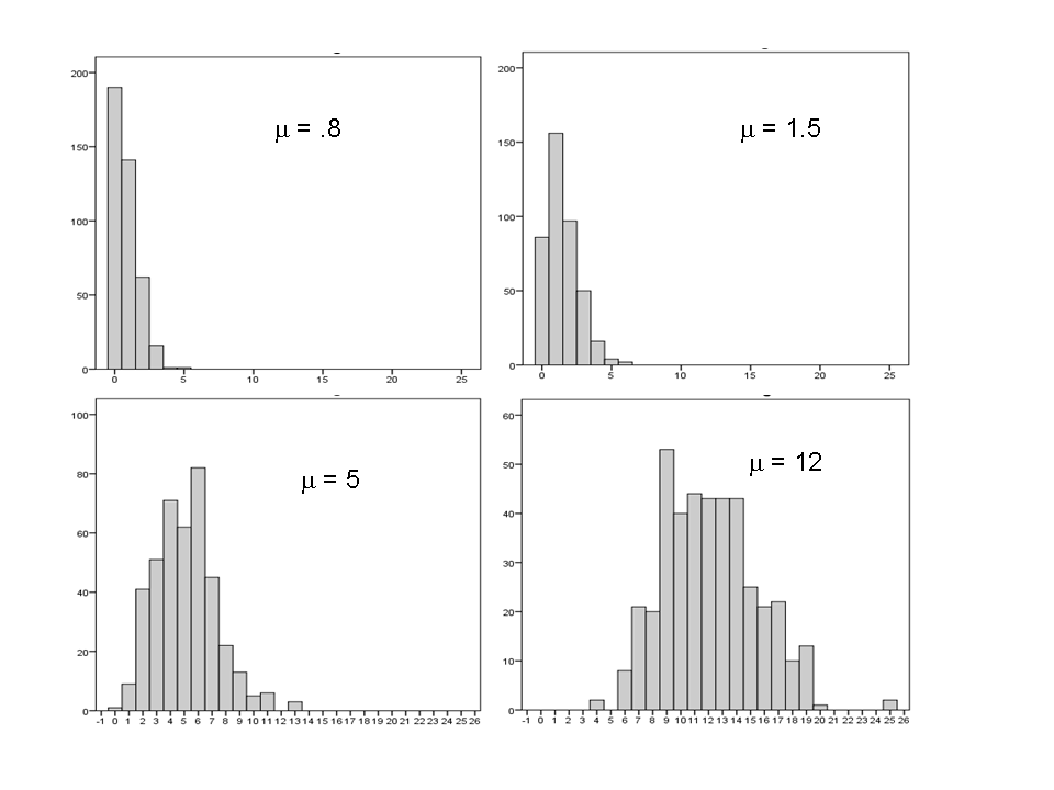
For example, a Poisson distribution with a low mean is highly skewed, with 0 as the mode. All the data are “pushed” up against 0, with a tail extending to the right. You can see an example in the upper left quadrant above.
But if the mean is larger, the distribution spreads out and becomes more symmetric. In fact, with a mean as high as 12, the distribution looks downright normal.
A Poisson distribution with a high enough mean approximates a normal distribution, even though technically, it is not.
One difference is that in the Poisson distribution the variance = the mean. In a normal distribution, these are two separate parameters. The value of one tells you nothing about the other.
So a Poisson distributed variable may look normal, but it won’t quite behave the same.
Can you treat it as normal?
In some cases, yes. You’ll still get reasonable parameter estimates and standard errors.
But don’t do it blindly. Check your assumptions. (You always do, right?)
If the distribution is too skewed or residual variance too heteroskedastic to assume normality, then no. Stick with a model that takes the true distribution into account.
*Edited 2/24/25 to fix some unclear wording about what discrete variables are.
A note on this. A few commenters pointed out that discrete variables don’t have to be whole numbers. Just a specific set of numbers.
And yes, that’s true. It’s the technical definition. And I do agree that sticking with technical definitions is important. So I fixed that.
I will add, though, that discrete numerical outcome variables that are not whole numbers are uncommon. I can’t remember ever seeing one in real data sets. (Not true for predictor variables!) That, of course, doesn’t mean they don’t exist or they aren’t common in some specific field.

Thanks for this. And for all your other little articles on things I should already know about but don’t really.
They are pitched just right for me.
They are just long enough, not interfering with my work.
I really enjoy reading them, you are a great teacher.
Right away: discrete doesn’t mean “a whole number”. Discrete means: takes particular values, changes abruptly as a function of the parameter set. The particular value that one associates with the steps in this change depends on the normalization and has nothing to do with the value being defined on a set of rational/natural numbers.
E.g.: a set {0.1, 2.0, 4.4} is a set of numbers that can correspond to a discrete variable, say, energy spectrum of an electron in an EM system. Why would one expect a by def discrete (!) variable like this to be defined on a set of whole numbers?? The same with, say, weight of humans in a data set, age… All those can be variables… It depends on your model.
I am trying to find mathematical formulas for the Poisson and Normal statistics to compare them side by side. I suspect they are similar with simple to explain differences. I will keep looking.
With thanks.
They’re not similar, though they do have a special relationship. Any textbook on theoretical stats will have the formulas.
You can find them clicking some of the links here: http://www.socr.ucla.edu/Applets.dir/NormalApprox2PoissonApplet.html
Thank you so much for this explanation! This sort of explanation was precisely what I was looking for!
Thanks for the helpful article. There’s a minor error though when you say that “discrete variables can only be whole numbers”. Technically speaking, a discrete variable is one in which its possible values are countable. For example, consider a variable X that can take any value in {0, 0.5, 1, 1.5, 2}. X is discrete, but not necessarily a whole number!
I just wanted to thank you for your daily Linked-in comments. They are a helpful service to the community, even for the highly trained and experienced among us. Sometimes it is refreshing to think about the simple things that may have slipped your mind and which have unexpectedly great depth because the first time you heard them, you yourself did not have great depth of skill or knowledge and so they just passed as facts into the back of your brain.
Totally agree with David’s comments. Its a day after the conference in where this became in my mind a highlight.