by Jeff Meyer, MBA, MPA
One of the most important concepts in data analysis is that the analysis needs to be appropriate for the scale of measurement of the variable. The focus of these decisions about scale tends to focus on levels of measurement: nominal, ordinal, interval, ratio.
These levels of measurement tell you about the amount of information in the variable. But there are other ways of distinguishing the scales that are also important and often overlooked.
For example, ratio-level variables can be of two types: continuous and discrete. Continuous variables can take on any value on a number line, whereas discrete variables can take on only integers.
This is important in statistics because we measure the probabilities differently for discrete and continuous distributions.
The probability of each value of a discrete random variable is described through a probability distribution. At its simplest, this is a list of all the values in the set and the probability of each value occurring.
But the probabilities of many discrete random variables follow patterns that can be described with a mathematical function. This function is called a probability mass function (pmf).
As you can imagine, there are numerous discrete probability distributions. A few of you may have heard of are Bernoulli, binomial, hypergeometric, discrete uniform, and Poisson. There are explicit criteria that determine which probability distribution is appropriate for a specific discrete random variable.
Count data are a good example. A count variable is discrete because it consists of non-negative integers. Even so, there is not one specific probability distribution that fits all count data sets.
The Poisson Distribution
The Poisson distribution often fits count data. It fits well when the mean of the variable is equal to its variance. So how do you determine that?
Run a summary of your variable in your statistical software package and compare the mean to the variance. If the standard deviation is listed instead of the variance, just square the standard deviation. If they are almost equal, then that’s a good sign.
You can also run a qqplot of your data against a Poisson distribution. Although we usually use these for normal distributions, you can do it with any of a number of distributions.
But many count variables fail these tests.
Below are two graphs generated with Poisson and negative binomial probability distribution functions. Each has 5,000 observations. The mean of the Poisson data is 2, the variance is 1.99, and the range is from 0 to 8. The mean of the negative binomial data is 2, the variance is 4.16, and the range is from 0 to 15.
The negative binomial distribution contains an extra parameter that allows the variance to be greater than the mean. If you tried to fit a data set with that mean and variance to a Poisson distribution, it would be considered overdispersed — not a good fit.
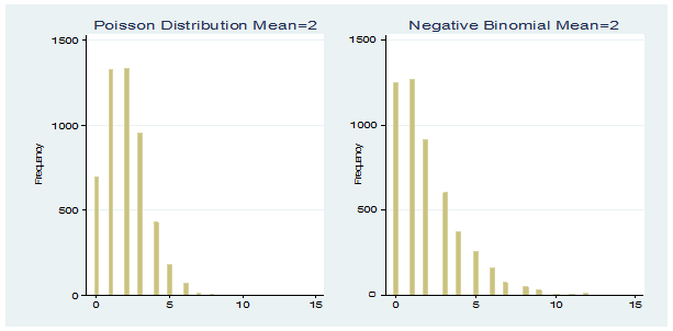
Notice that there is a probability for each non-negative value on the x axis, beginning with zero. A Poisson or negative binomial random number generator will only create non-negative integers.
The Normal Distribution
If the mean of a Poisson or negative binomial variable is high enough, it will be symmetric and bell-shaped. It will look like a normal distribution, except for one key distinction—normal variables are truly continuous, not discrete. They can take on any possible value.
As a result, there are an infinite number of values (2.30546 is a different value than 2.30547). It makes no sense to calculate the probability that X is any exact value in a continuous variable. That probability is infinitesimal, a value approaching zero.
With continuous variables, the probability of a value falling within a range is calculated instead. For example, there is a 95% probability that a value from a normal distribution will fall within 1.96 standard deviations of the mean of that distribution.
To show you the difference, I created a set of 5,000 random values from a normal distribution with a mean and variance of 2. The range of the data is -2.512433 to 7.461702. Included next to its graph is the graph of the Poisson variable with a mean and variance of 2.
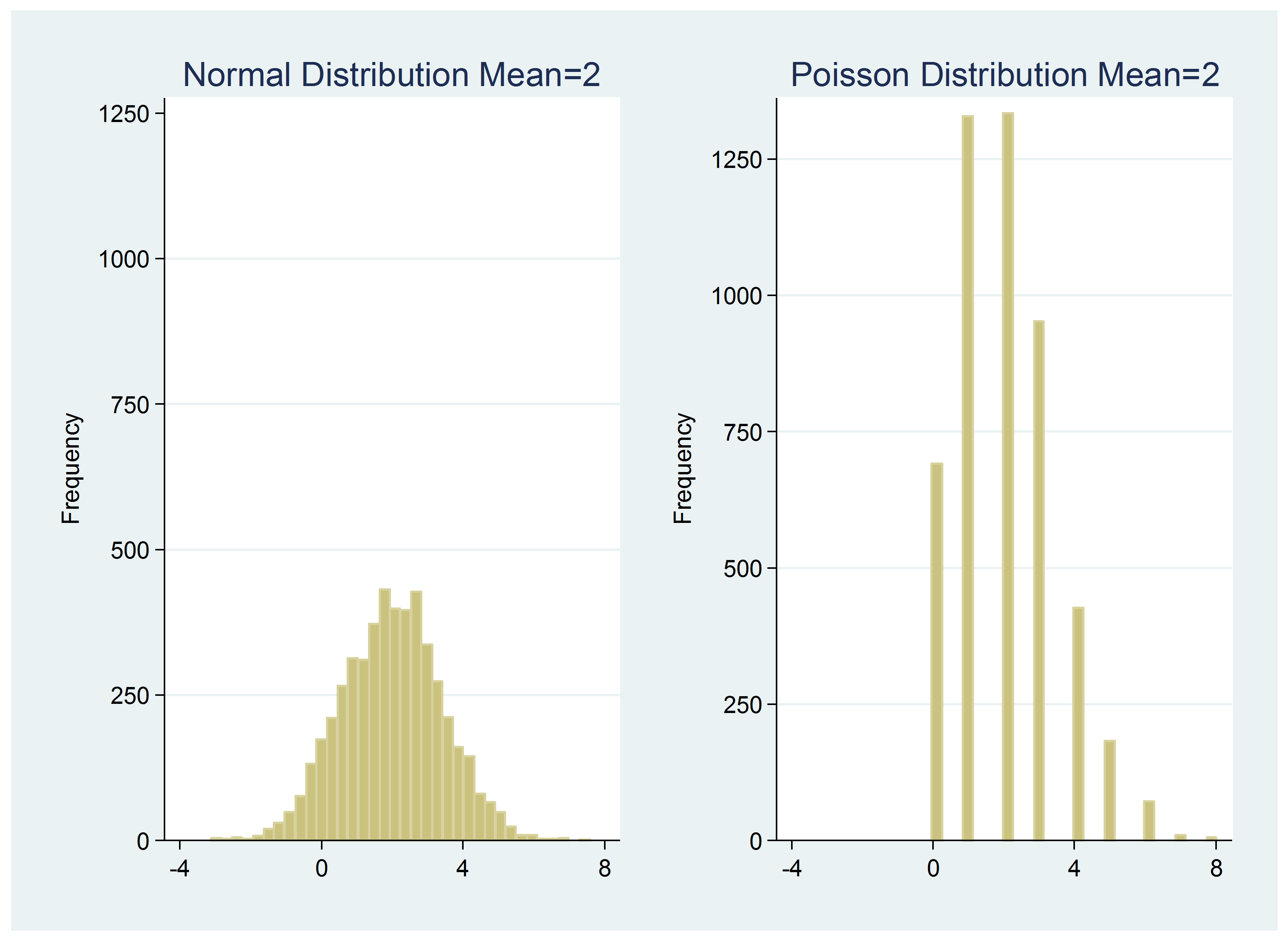
Note the following:
The ranges differ a lot (values are less than zero for the continuous variable).
There is a large difference in the number of unique observations (4,999 for the continuous set and 9 for the discrete Poisson set).
The take-away here?
Examine your outcome variable to determine whether it is discrete or continuous. If it is discrete, find the probability distribution function that best matches its make-up.
Jeff Meyer is a statistical consultant with The Analysis Factor, a stats mentor for Statistically Speaking membership, and a workshop instructor. Read more about Jeff here.

Leave a Reply