In my last blog post we fitted a generalized linear model to count data using a Poisson error structure.
We found, however, that there was over-dispersion in the data – the variance was larger than the mean in our dependent variable.
In my last blog post we fitted a generalized linear model to count data using a Poisson error structure.
We found, however, that there was over-dispersion in the data – the variance was larger than the mean in our dependent variable.
In my last couple of articles (Part 4, Part 5), I demonstrated a logistic regression model with binomial errors on binary data in R’s glm() function.
But one of wonderful things about glm() is that it is so flexible. It can run so much more than logistic regression models.
The flexibility, of course, also means that you have to tell it exactly which model you want to run, and how.
In fact, we can use generalized linear models to model count data as well.
In such data the errors may well be distributed non-normally and the variance usually increases with the mean values.
As with binary data, we use the glm() command, but this time we specify a Poisson error distribution and the logarithm as the link function.
The natural log is the default link function for the Poisson error distribution. It works well for count data as it forces all of the predicted values to be positive.
In the following example we fit a generalized linear model to count data using a Poisson error structure. The data set consists of counts of high school students diagnosed with an infectious disease within a period of days from an initial outbreak.
cases <-
structure(list(Days = c(1L, 2L, 3L, 3L, 4L, 4L, 4L, 6L, 7L, 8L,
8L, 8L, 8L, 12L, 14L, 15L, 17L, 17L, 17L, 18L, 19L, 19L, 20L,
23L, 23L, 23L, 24L, 24L, 25L, 26L, 27L, 28L, 29L, 34L, 36L, 36L,
42L, 42L, 43L, 43L, 44L, 44L, 44L, 44L, 45L, 46L, 48L, 48L, 49L,
49L, 53L, 53L, 53L, 54L, 55L, 56L, 56L, 58L, 60L, 63L, 65L, 67L,
67L, 68L, 71L, 71L, 72L, 72L, 72L, 73L, 74L, 74L, 74L, 75L, 75L,
80L, 81L, 81L, 81L, 81L, 88L, 88L, 90L, 93L, 93L, 94L, 95L, 95L,
95L, 96L, 96L, 97L, 98L, 100L, 101L, 102L, 103L, 104L, 105L,
106L, 107L, 108L, 109L, 110L, 111L, 112L, 113L, 114L, 115L),
    Students = c(6L, 8L, 12L, 9L, 3L, 3L, 11L, 5L, 7L, 3L, 8L,
    4L, 6L, 8L, 3L, 6L, 3L, 2L, 2L, 6L, 3L, 7L, 7L, 2L, 2L, 8L,
    3L, 6L, 5L, 7L, 6L, 4L, 4L, 3L, 3L, 5L, 3L, 3L, 3L, 5L, 3L,
    5L, 6L, 3L, 3L, 3L, 3L, 2L, 3L, 1L, 3L, 3L, 5L, 4L, 4L, 3L,
    5L, 4L, 3L, 5L, 3L, 4L, 2L, 3L, 3L, 1L, 3L, 2L, 5L, 4L, 3L,
    0L, 3L, 3L, 4L, 0L, 3L, 3L, 4L, 0L, 2L, 2L, 1L, 1L, 2L, 0L,
    2L, 1L, 1L, 0L, 0L, 1L, 1L, 2L, 2L, 1L, 1L, 1L, 1L, 0L, 0L,
    0L, 1L, 1L, 0L, 0L, 0L, 0L, 0L)), .Names = c("Days", "Students"
), class = "data.frame", row.names = c(NA, -109L))

attach(cases)

head(cases)
    Days Students
1    1      6
2    2      8
3    3     12
4    3      9
5    4      3
6    4      3
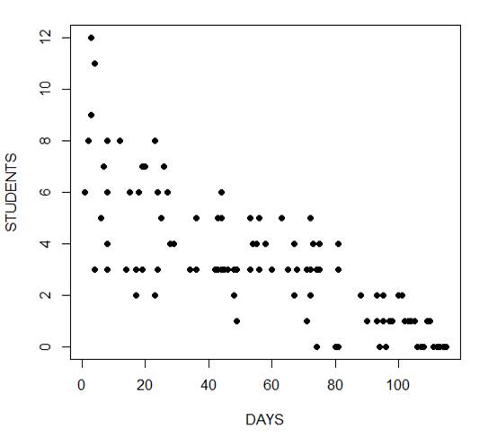
The mean and variance are different (actually, the variance is greater). Now we plot the data.
plot(Days, Students, xlab = "DAYS", ylab = "STUDENTS", pch = 16)
Now we fit the glm, specifying the Poisson distribution by including it as the second argument.
model1 <- glm(Students ~ Days, poisson) summary(model1) Call: glm(formula = Students ~ Days, family = poisson) Deviance Residuals: Min 1Q Median 3Q Max -2.00482 -0.85719 -0.09331 0.63969 1.73696 Coefficients: Estimate Std. Error z value Pr(>|z|)
(Intercept)  1.990235   0.083935   23.71   <2e-16 ***
Days        -0.017463   0.001727  -10.11   <2e-16 ***
---
Signif. codes:  0 ‘***’ 0.001 ‘**’ 0.01 ‘*’ 0.05 ‘.’ 0.1 ‘ ’ 1

(Dispersion parameter for poisson family taken to be 1)

    Null deviance: 215.36  on 108  degrees of freedom
Residual deviance: 101.17  on 107  degrees of freedom
AIC: 393.11

Number of Fisher Scoring iterations: 5
The negative coefficient for Days indicates that as days increase, the mean number of students with the disease is smaller.
This coefficient is highly significant (p < 2e-16).
We also see that the residual deviance is greater than the degrees of freedom, so that we have over-dispersion. This means that there is extra variance not accounted for by the model or by the error structure.
This is a very important model assumption, so in my next article we will re-fit the model using quasi poisson errors.
****
See our full R Tutorial Series and other blog posts regarding R programming.
About the Author: David Lillis has taught R to many researchers and statisticians. His company, Sigma Statistics and Research Limited, provides both on-line instruction and face-to-face workshops on R, and coding services in R. David holds a doctorate in applied statistics.
Count variables are common dependent variables in many fields. For example:
Although they are numerical and look like they should work in linear models, they often don’t.
Not only are they discrete instead of continuous (you can’t have 7.2 eggs hatching!), they can’t go below 0. And since 0 is often the most common value, they’re often highly skewed — so skewed, in fact, that transformations don’t work.
There are, however, generalized linear models that work well for count data. They take into account the specific issues inherent in count data. They should be accessible to anyone who is familiar with linear or logistic regression.
In this webinar, we’ll discuss the different model options for count data, including how to figure out which one works best. We’ll go into detail about how the models are set up, some key statistics, and how to interpret parameter estimates.
Note: This training is an exclusive benefit to members of the Statistically Speaking Membership Program and part of the Stat’s Amore Trainings Series. Each Stat’s Amore Training is approximately 90 minutes long.

Karen Grace-Martin helps statistics practitioners gain an intuitive understanding of how statistics is applied to real data in research studies.
She has guided and trained researchers through their statistical analysis for over 15 years as a statistical consultant at Cornell University and through The Analysis Factor. She has master’s degrees in both applied statistics and social psychology and is an expert in SPSS and SAS.
Just head over and sign up for Statistically Speaking.
You'll get access to this training webinar, 130+ other stats trainings, a pathway to work through the trainings that you need — plus the expert guidance you need to build statistical skill with live Q&A sessions and an ask-a-mentor forum.
Linear, Logistic, Tobit, Cox, Poisson, Zero Inflated… The list of regression models goes on and on before you even get to things like ANCOVA or Linear Mixed Models.
In this webinar, we will explore types of regression models, how they differ, how they’re the same, and most importantly, when to use each one.
Note: This training is an exclusive benefit to members of the Statistically Speaking Membership Program and part of the Stat’s Amore Trainings Series. Each Stat’s Amore Training is approximately 90 minutes long.
Karen Grace-Martin helps statistics practitioners gain an intuitive understanding of how statistics is applied to real data in research studies.
She has guided and trained researchers through their statistical analysis for over 15 years as a statistical consultant at Cornell University and through The Analysis Factor. She has master’s degrees in both applied statistics and social psychology and is an expert in SPSS and SAS.
Just head over and sign up for Statistically Speaking. You'll get access to this training webinar, 130+ other stats trainings, a pathway to work through the trainings that you need — plus the expert guidance you need to build statistical skill with live Q&A sessions and an ask-a-mentor forum.Not a Member Yet?
It’s never too early to set yourself up for successful analysis with support and training from expert statisticians.
1. For a general overview of modeling count variables, you can get free access to the video recording of one of my The Craft of Statistical Analysis Webinars:
Poisson and Negative Binomial for Count Outcomes
2. One of my favorite books on Categorical Data Analysis is:
Long, J. Scott. (1997). Regression models for Categorical and Limited Dependent Variables. Sage Publications.
It’s moderately technical, but written with social science researchers in mind. It’s so well written, it’s worth it. It has a section specifically about Zero Inflated Poisson and Zero Inflated Negative Binomial regression models.
3. Slightly less technical, but most useful only if you use Stata is >Regression Models for Categorical Dependent Variables Using Stata, by J. Scott Long and Jeremy Freese.
4. UCLA’s ATS Statistical Software Consulting Group has some nice examples of Zero-Inflated Poisson and other models in various software packages.
There are quite a few types of outcome variables that will never meet ordinary linear model’s assumption of normally distributed residuals. A non-normal outcome variable can have normally distribued residuals, but it does need to be continuous, unbounded, and measured on an interval or ratio scale. Categorical outcome variables clearly don’t fit this requirement, so it’s easy to see that an ordinary linear model is not appropriate. Neither do count variables. It’s less obvious, because they are measured on a ratio scale, so it’s easier to think of them as continuous, or close to it. But they’re neither continuous or unbounded, and this really affects assumptions.
Continuous variables measure how much. Count variables measure how many. Count variables can’t be negative—0 is the lowest possible value, and they’re often skewed–so severly that 0 is by far the most common value. And they’re discrete, not continuous. All those jokes about the average family having 1.3 children have a ring of truth in this context.
Count variables often follow a Poisson or one of its related distributions. The Poisson distribution assumes that each count is the result of the same Poisson process—a random process that says each counted event is independent and equally likely. If this count variable is used as the outcome of a regression model, we can use Poisson regression to estimate how predictors affect the number of times the event occurred.
But the Poisson model has very strict assumptions. One that is often violated is that the mean equals the variance. When the variance is too large because there are many 0s as well as a few very high values, the negative binomial model is an extension that can handle the extra variance.
But sometimes it’s just a matter of having too many zeros than a Poisson would predict. In this case, a better solution is often the Zero-Inflated Poisson (ZIP) model. (And when extra variation occurs too, its close relative is the Zero-Inflated Negative Binomial model).
ZIP models assume that some zeros occurred by a Poisson process, but others were not even eligible to have the event occur. So there are two processes at work—one that determines if the individual is even eligible for a non-zero response, and the other that determines the count of that response for eligible individuals.
The tricky part is either process can result in a 0 count. Since you can’t tell which 0s were eligible for a non-zero count, you can’t tell which zeros were results of which process. The ZIP model fits, simultaneously, two separate regression models. One is a logistic or probit model that models the probability of being eligible for a non-zero count. The other models the size of that count.
Both models use the same predictor variables, but estimate their coefficients separately. So the predictors can have vastly different effects on the two processes.
But a ZIP model requires it be theoretically plausible that some individuals are ineligible for a count. For example, consider a count of the number of disciplinary incidents in a day in a youth detention center. True, there may be some youth who would never instigate an incident, but the unit of observation in this case is the center. It is hard to imagine a situation in which a detention center would have no possibility of any incidents, even if they didn’t occur on some days.
Compare that to the number of alcoholic drinks consumed in a day, which could plausibly be fit with a ZIP model. Some participants do drink alcohol, but will have consumed 0 that day, by chance. But others just do not drink alcohol, so will never have a non-zero response. The ZIP model can determine which predictors affect the probability of being an alcohol consumer and which predictors affect how many drinks the consumers consume. They may not be the same predictors for the two models, or they could even have opposite effects on the two processes.