principal component analysis

One of the many confusing issues in statistics is the confusion between Principal Component Analysis (PCA) and Factor Analysis (FA).

They are very similar in many ways, so it’s not hard to see why they’re so often confused. They appear to be different varieties of the same analysis rather than two different methods. Yet there is a fundamental difference between them that has huge effects on how to use them.

(Like donkeys and zebras. They seem to differ only by color until you try to ride one).

Both are data reduction techniques—they allow you to capture the variance in variables in a smaller set.

Both are usually run in stat software using the same procedure, and the output looks pretty much the same.

The steps you take to run them are the same—extraction, interpretation, rotation, choosing the number of factors or components.

Despite all these similarities, there is a fundamental difference between them: PCA is a linear combination of variables; Factor Analysis is a measurement model of a latent variable.

Principal Component Analysis

PCA’s approach to data reduction is to create one or more index variables from a larger set of measured variables. It does this using a linear combination (basically a weighted average) of a set of variables. The created index variables are called components.

The whole point of the PCA is to figure out how to do this in an optimal way: the optimal number of components, the optimal choice of measured variables for each component, and the optimal weights.

The picture below shows what a PCA is doing to combine 4 measured (Y) variables into a single component, C. You can see from the direction of the arrows that the Y variables contribute to the component variable. The weights allow this combination to emphasize some Y variables more than others.

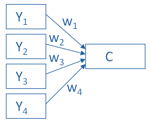
This model can be set up as a simple equation:

C = w₁(Y₁) + w₂(Y₂) + w₃(Y₃) + w₄(Y₄)

Factor Analysis

A Factor Analysis approaches data reduction in a fundamentally different way. It is a model of the measurement of a latent variable. This latent variable cannot be directly measured with a single variable (think: intelligence, social anxiety, soil health).  Instead, it is seen through the relationships it causes in a set of Y variables.

For example, we may not be able to directly measure social anxiety. But we can measure whether social anxiety is high or low with a set of variables like “I am uncomfortable in large groups” and “I get nervous talking with strangers.” People with high social anxiety will give similar high responses to these variables because of their high social anxiety. Likewise, people with low social anxiety will give similar low responses to these variables because of their low social anxiety.

The measurement model for a simple, one-factor model looks like the diagram below. It’s counter intuitive, but F, the latent Factor, is causing the responses on the four measured Y variables. So the arrows go in the opposite direction from PCA. Just like in PCA, the relationships between F and each Y are weighted, and the factor analysis is figuring out the optimal weights.

In this model we have is a set of error terms. These are designated by the u’s. This is the variance in each Y that is unexplained by the factor.

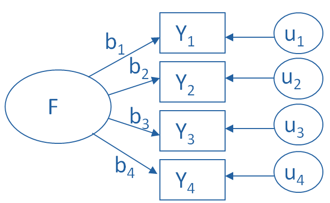
You can literally interpret this model as a set of regression equations:

Y₁ = b₁*F + u₁
Y₂ = b₂*F + u₂
Y₃ = b₃*F + u₃
Y₄ = b₄*F + u₄

As you can probably guess, this fundamental difference has many, many implications. These are important to understand if you’re ever deciding which approach to use in a specific situation.

Go to the next article or see the full series on Easy-to-Confuse Statistical Concepts

26 comments

Here’s a question I get pretty often: In Principal Component Analysis, can loadings be negative and positive?

Answer: Yes.

Recall that in PCA, we are creating one index variable (or a few) from a set of variables. You can think of this index variable as a weighted average of the original variables.

The loadings are the correlations between the variables and the component. We compute the weights in the weighted average from these loadings.

The goal of the PCA is to come up with optimal weights. “Optimal” means we’re capturing as much information in the original variables as possible, based on the correlations among those variables.

So if all the variables in a component are positively correlated with each other, all the loadings will be positive.

But if there are some negative correlations among the variables, some of the loadings will be negative too.

An Example of Negative Loadings in Principal Component Analysis

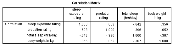
Here’s a simple example that we used in our Principal Component Analysis webinar. We want to combine four variables about mammal species into a single component.

The variables are weight, a predation rating, amount of exposure while sleeping, and the total number of hours an animal sleeps each day.

If you look at the correlation matrix, total hours of sleep correlates negatively with the other 3 variables. Those other three are all positively correlated.

It makes sense — species that sleep more tend to be smaller, less exposed while sleeping, and less prone to predation. Species that are high on these three variables must not be able to afford much sleep.

Think bats vs. zebras.

Likewise, the PCA with one component has positive loadings for three of the variables and a negative loading for hours of sleep.

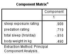
Species with a high component score will be those with high weight, high predation rating, high sleep exposure, and low hours of sleep.

1 comment

Principal Component Analysis is really, really useful.

You use it to create a single index variable from a set of correlated variables.

In fact, the very first step in Principal Component Analysis is to create a correlation matrix (a.k.a., a table of bivariate correlations). The rest of the analysis is based on this correlation matrix.

You don’t usually see this step — it happens behind the scenes in your software.

Most PCA procedures calculate that first step using only one type of correlations: Pearson.

And that can be a problem. Pearson correlations assume all variables are normally distributed. That means they have to be truly (more…)

20 comments

One common reason for running Principal Component Analysis (PCA) or Factor Analysis (FA) is variable reduction.

In other words, you may start with a 10-item scale meant to measure something like Anxiety, which is difficult to accurately measure with a single question.

You could use all 10 items as individual variables in an analysis–perhaps as predictors in a regression model.

But you’d end up with a mess.

Not only would you have trouble interpreting all those coefficients, but you’re likely to have multicollinearity problems.

And most importantly, you’re not interested in the effect of each of those individual 10 items on your (more…)

15 comments

I received a question recently about R Commander, a free R package.

R Commander overlays a menu-based interface to R, so just like SPSS or JMP, you can run analyses using menus.  Nice, huh?

The question was whether R Commander does everything R does, or just a small subset.

Unfortunately, R Commander can’t do everything R does. Not even close.

But it does a lot. More than just the basics.

So I thought I would show you some of the things R Commander can do entirely through menus–no programming required, just so you can see just how unbelievably useful it is.

Since R commander is a free R package, it can be installed easily through R! Just type install.packages("Rcmdr") in the command line the first time you use it, then type library("Rcmdr") each time you want to launch the menus.

Data Sets and Variables

Import data sets from other software:

• SPSS
• Stata
• Excel
• Minitab
• Text
• SAS Xport
  

Define Numerical Variables as categorical and label the values

Open the data sets that come with R packages

Merge Data Sets

Edit and show the data in a data spreadsheet

Personally, I think that if this was all R Commander did, it would be incredibly useful. These are the types of things I just cannot remember all the commands for, since I just don’t use R often enough.

Data Analysis

Yes, R Commander does many of the simple statistical tests you’d expect:

• Chi-square tests
• Paired and Independent Samples t-tests
• Tests of Proportions
• Common nonparametrics, like Friedman, Wilcoxon, and Kruskal-Wallis tests
• One-way ANOVA and simple linear regression

What is surprising though, is how many higher-level statistics and models it runs:

• Hierarchical and K-Means Cluster analysis (with 7 linkage methods and 4 options of distance measures)
• Principal Components and Factor Analysis
• Linear Regression (with model selection, influence statistics, and multicollinearity diagnostic options, among others)
• Logistic regression for binary, ordinal, and multinomial responses
• Generalized linear models, including Gamma and Poisson models

In other words–you can use R Commander to run in R most of the analyses that most researchers need.

Graphs

A sample of the types of graphs R Commander creates in R without you having to write any code:

• QQ Plots
• Scatter plots
• Histograms
• Box Plots
• Bar Charts

The nice part is that it does not only do simple versions of these plots.  You can, for example, add regression lines to a scatter plot or run histograms by a grouping factor.

If you’re ready to get started practicing, click here to learn about making scatterplots in R commander, or click here to learn how to use R commander to sample from a uniform distribution.

4 comments

Principal Component Analysis (PCA) is a handy statistical tool to always have available in your data analysis tool belt.

It’s a data reduction technique, which means it’s a way of capturing the variance in many variables in a smaller, easier-to-work-with set of variables.

There are many, many details involved, though, so here are a few things to remember as you run your PCA.

1. The goal of PCA is to summarize the correlations among a set of observed variables with a smaller set of linear (more…)

7 comments