 Is it really ok to treat Likert items as continuous?
 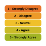 And can you just decide to combine Likert items to make a scale? Likert-type data is extremely common—and so are questions like these about how to analyze it appropriately. (more…)
ANOVA
Member Training: Analyzing Likert Scale Data
August 31st, 2022 by TAF Support
When Linear Models Don’t Fit Your Data, Now What?
June 20th, 2022 by Karen Grace-Martin
When your dependent variable is not continuous, unbounded, and measured on an interval or ratio scale, linear models don’t fit. The data just will not meet the assumptions of linear models. But there’s good news, other models exist for many types of dependent variables.
Today I’m going to go into more detail about 6 common types of dependent variables that are either discrete, bounded, or measured on a nominal or ordinal scale and the tests that work for them instead. Some are all of these.
Specifying Fixed and Random Factors in Mixed Models
January 10th, 2022 by Karen Grace-Martin
One of the difficult decisions in mixed modeling is deciding which factors are fixed and which are random. And as difficult as it is, it’s also very important. Correctly specifying the fixed and random factors of the model is vital to obtain accurate analyses.
Now, you may be thinking of the fixed and random effects in the model, rather than the factors themselves, as fixed or random. If so, remember that each term in the model (factor, covariate, interaction or other multiplicative term) has an effect. We’ll come back to how the model measures the effects for fixed and random factors.
Sadly, the definitions in many texts don’t help much with decisions to specify factors as fixed or random. Textbook examples are often artificial and hard to apply to the real, messy data you’re working with.
Here’s the real kicker. The same factor can often be fixed or random, depending on the researcher’s objective. (more…)
Member Training: Classic Experimental Designs
October 29th, 2021 by Kim Love
 Have you ever wondered why there are so many different types of experimental designs, and how a researcher would go about choosing among them to best address their research questions? (more…)
Member Training: ANOVA Post-hoc Tests: Practical Considerations
October 1st, 2021 by TAF Support
Post-hoc tests, pairwise or other linear contrasts, are typical in an analysis of variance (ANOVA) setting to understand which group means differ. They incorporate p-value adjustments to avoid concluding that group means differ when they actually do not. There are several adjustments that can be considered for conducting multiple post-hoc tests, including single-step and stepwise adjustments. (more…)
Why report estimated marginal means?
August 18th, 2021 by Karen Grace-Martin
Updated 8/18/2021
I recently was asked whether to report means from descriptive statistics or from the Estimated Marginal Means with SPSS GLM.
The short answer: Report the Estimated Marginal Means (almost always).
To understand why and the rare case it doesn’t matter, let’s dig in a bit with a longer answer.
First, a marginal mean is the mean response for each category of a factor, adjusted for any other variables in the model (more on this later).
Just about any time you include a factor in a linear model, you’ll want to report the mean for each group. The F test of the model in the ANOVA table will give you a p-value for the null hypothesis that those means are equal. And that’s important.
But you need to see the means and their standard errors to interpret the results. The difference in those means is what measures the effect of the factor. While that difference can also appear in the regression coefficients, looking at the means themselves give you a context and makes interpretation more straightforward. This is especially true if you have interactions in the model.
Some basic info about marginal means
- In SPSS menus, they are in the Options button and in SPSS’s syntax they’re EMMEANS.
- These are called LSMeans in SAS, margins in Stata, and emmeans in R’s emmeans package.
- Although I’m talking about them in the context of linear models, all the software has them in other types of models, including linear mixed models, generalized linear models, and generalized linear mixed models.
- They are also called predicted means, and model-based means. There are probably a few other names for them, because that’s what happens in statistics.
When marginal means are the same as observed means
Let’s consider a few different models. In all of these, our factor of interest, X, is a categorical predictor for which we’re calculating Estimated Marginal Means. We’ll call it the Independent Variable (IV).
Model 1: No other predictors
If you have just a single factor in the model (a one-way anova), marginal means and observed means will be the same.
Observed means are what you would get if you simply calculated the mean of Y for each group of X.
Model 2: Other categorical predictors, and all are balanced
Likewise, if you have other factors in the model, if all those factors are balanced, the estimated marginal means will be the same as the observed means you got from descriptive statistics.
Model 3: Other categorical predictors, unbalanced
Now things change. The marginal mean for our IV is different from the observed mean. It’s the mean for each group of the IV, averaged across the groups for the other factor.
When you’re observing the category an individual is in, you will pretty much never get balanced data. Even when you’re doing random assignment, balanced groups can be hard to achieve.
In this situation, the observed means will be different than the marginal means. So report the marginal means. They better reflect the main effect of your IV—the effect of that IV, averaged across the groups of the other factor.
Model 4: A continuous covariate
When you have a covariate in the model the estimated marginal means will be adjusted for the covariate. Again, they’ll differ from observed means.
It works a little bit differently than it does with a factor. For a covariate, the estimated marginal mean is the mean of Y for each group of the IV at one specific value of the covariate.
By default in most software, this one specific value is the mean of the covariate. Therefore, you interpret the estimated marginal means of your IV as the mean of each group at the mean of the covariate.
This, of course, is the reason for including the covariate in the model–you want to see if your factor still has an effect, beyond the effect of the covariate. You are interested in the adjusted effects in both the overall F-test and in the means.
If you just use observed means and there was any association between the covariate and your IV, some of that mean difference would be driven by the covariate.
For example, say your IV is the type of math curriculum taught to first graders. There are two types. And say your covariate is child’s age, which is related to the outcome: math score.
It turns out that curriculum A has slightly older kids and a higher mean math score than curriculum B. Observed means for each curriculum will not account for the fact that the kids who received that curriculum were a little older. Marginal means will give you the mean math score for each group at the same age. In essence, it sets Age at a constant value before calculating the mean for each curriculum. This gives you a fairer comparison between the two curricula.
But there is another advantage here. Although the default value of the covariate is its mean, you can change this default. This is especially helpful for interpreting interactions, where you can see the means for each group of the IV at both high and low values of the covariate.
In SPSS, you can change this default using syntax, but not through the menus.
For example, in this syntax, the EMMEANS statement reports the marginal means of Y at each level of the categorical variable X at the mean of the Covariate V.
UNIANOVA Y BY X WITH V
/INTERCEPT=INCLUDE
/EMMEANS=TABLES(X) WITH(V=MEAN)
/DESIGN=X V.
If instead, you wanted to evaluate the effect of X at a specific value of V, say 50, you can just change the EMMEANS statement to:
/EMMEANS=TABLES(X) WITH(V=50)
Another good reason to use syntax.