by Maike Rahn, PhD
When are factor loadings not strong enough?
Once you run a factor analysis and think you have some usable results, it’s time to eliminate variables that are not “strong” enough. They are usually the ones with low factor loadings, although additional criteria should be considered before taking out a variable.
As a rule of thumb, your variable should have a rotated factor loading of at least |0.4| (meaning ≥ +.4 or ≤ –.4) onto one of the factors in order to be considered important. (more…)

We were recently fortunate to host a free The Craft of Statistical Analysis Webinar with guest presenter David Lillis. As usual, we had hundreds of attendees and didn’t get through all the questions. So David has graciously agreed to answer questions here.
If you missed the live webinar, you can download the recording here: Ten Data Analysis Tips in R.
Q: Is the M=structure(.list(.., class = “data.frame) the same as M=data.frame(..)? Is there some reason to prefer to use structure(list, … ,) as opposed to M=data.frame?
A: They are not the same. The structure( .. .) syntax is a short-hand way of storing a data set. If you have a data set called M, then the command dput(M) provides a shorthand way of storing the dataset. You can then reconstitute it later as follows: M <- structure( . . . .). Try it for yourselves on a rectangular dataset. For example, start off with (more…)
Have you ever been told you need to run a mixed (aka: multilevel) model and been thrown off by all the new vocabulary?
It happened to me when I first started my statistical consulting job, oh so many years ago. I had learned mixed models in an ANOVA class, so I had a pretty good grasp on many of the concepts.
But when I started my job, SAS had just recently come out with Proc Mixed, and it was the first time I had to actually implement a true multilevel model. I was out of school, so I had to figure it out on the job.
And even with my background, I had a pretty steep learning curve to get to a point where it made sense. Sure, I was able to figure out the steps, but there are some pretty tricky situations and complicated designs out there.
To implement it well, you need a good understanding of the big picture, and how the small parts fit into it. (more…)
One area in statistics where I see conflicting advice is how to analyze pre-post data. I’ve seen this myself in consulting. A few years ago, I received a call from a distressed client. Let’s call her Nancy.
Nancy had asked for advice about how to run a repeated measures analysis. The advisor told Nancy that actually, a repeated measures analysis was inappropriate for her data.
Nancy was sure repeated measures was appropriate. This advice led her to fear that she had grossly misunderstood a very basic tenet in her statistical training.
The Study Design
Nancy had measured a response variable at two time points for two groups. The intervention group received a treatment and a control group did not. Participants were randomly assigned to one of the two groups.
The researcher measured each participant before and after the intervention.
Analyzing the Pre-Post Data
Nancy was sure that this was a classic repeated measures experiment. It has (more…)
In Part 2 of this series, we created two variables and used the lm() command to perform a least squares regression on them, treating one of them as the dependent variable and the other as the independent variable. Here they are again.
height = c(176, 154, 138, 196, 132, 176, 181, 169, 150, 175)
bodymass = c(82, 49, 53, 112, 47, 69, 77, 71, 62, 78)
Today we learn how to obtain useful diagnostic information about a regression model and then how to draw residuals on a plot. As before, we perform the regression.
lm(height ~ bodymass)
Call:
lm(formula = height ~ bodymass)
Coefficients:
(Intercept) bodymass
98.0054 0.9528
Now let’s find out more about the regression. First, let’s store the regression model as an object called mod and then use the summary() command to learn about the regression.
mod <- lm(height ~ bodymass)
summary(mod)
Here is what R gives you.
Call:
lm(formula = height ~ bodymass)
Residuals:
Min 1Q Median 3Q Max
-10.786 -8.307 1.272 7.818 12.253
Coefficients:
Estimate Std. Error t value Pr(>|t|)
(Intercept) 98.0054 11.7053 8.373 3.14e-05 ***
bodymass 0.9528 0.1618 5.889 0.000366 ***
Signif. codes: 0 ‘***’ 0.001 ‘**’ 0.01 ‘*’ 0.05 ‘.’ 0.1 ‘ ’ 1
Residual standard error: 9.358 on 8 degrees of freedom
Multiple R-squared: 0.8126, Adjusted R-squared: 0.7891
F-statistic: 34.68 on 1 and 8 DF, p-value: 0.0003662
R has given you a great deal of diagnostic information about the regression. The most useful of this information are the coefficients themselves, the Adjusted R-squared, the F-statistic and the p-value for the model.
Now let’s use R’s predict() command to create a vector of fitted values.
regmodel <- predict(lm(height ~ bodymass))
regmodel
Here are the fitted values:
1 2 3 4 5 6 7 8 9 10
176.1334 144.6916 148.5027 204.7167 142.7861 163.7472 171.3695 165.6528 157.0778 172.3222
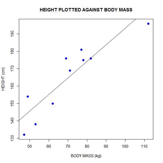
Now let’s plot the data and regression line again.
plot(bodymass, height, pch = 16, cex = 1.3, col = "blue", main = "HEIGHT PLOTTED AGAINST BODY MASS", xlab = "BODY MASS (kg)", ylab = "HEIGHT (cm)")
abline(lm(height ~ bodymass))
We can plot the residuals using R’s for loop and a subscript k that runs from 1 to the number of data points. We know that there are 10 data points, but if we do not know the number of data we can find it using the length() command on either the height or body mass variable.
npoints <- length(height)

npoints
[1] 10
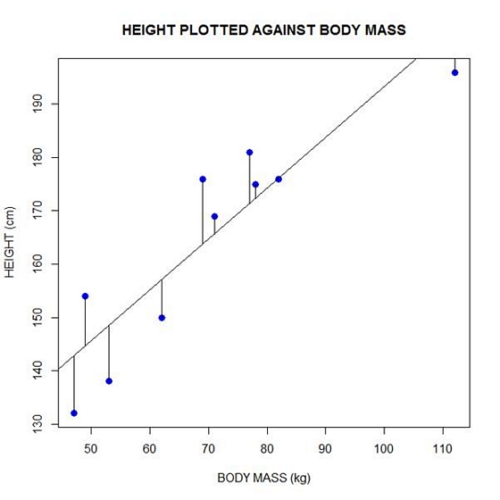
Now let’s implement the loop and draw the residuals (the differences between the observed data and the corresponding fitted values) using the lines() command. Note the syntax we use to draw in the residuals.
for (k in 1: npoints) lines(c(bodymass[k], bodymass[k]), c(height[k], regmodel[k]))
Here is our plot, including the residuals.
In part 4 we will look at more advanced aspects of regression models and see what R has to offer.
About the Author: David Lillis has taught R to many researchers and statisticians. His company, Sigma Statistics and Research Limited, provides both on-line instruction and face-to-face workshops on R, and coding services in R. David holds a doctorate in applied statistics.
See our full R Tutorial Series and other blog posts regarding R programming.
If you’ve ever worked with multilevel models, you know that they are an extension of linear models. For a researcher learning them, this is both good and bad news.
The good side is that many of the concepts, calculations, and results are familiar. The down side of the extension is that everything is more complicated in multilevel models.
This includes power and sample size calculations. (more…)