If you have a categorical predictor variable that you plan to use in a regression analysis in SPSS, there are a couple ways to do it.
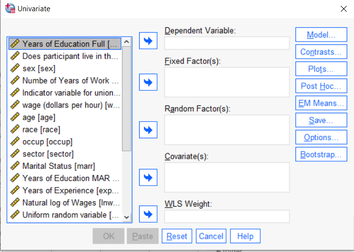
You can use the SPSS Regression procedure. Or you can use SPSS General Linear Model–>Univariate, which I discuss here. If you use Syntax, it’s the UNIANOVA command.
The big question in SPSS GLM is what goes where. As I’ve detailed in another post, any continuous independent variable goes into covariates. And don’t use random factors at all unless you really know what you’re doing.
So the question is what to do with your categorical variables. You have two choices, and each has advantages and disadvantages.
The easiest is to put categorical variables in Fixed Factors. SPSS GLM will dummy code those variables for you, which is quite convenient if your categorical variable has more than two categories.
However, there are some defaults you need to be aware of that may or may not make this a good choice.
The dummy coding reference group default
SPSS GLM always makes the reference group the one that comes last alphabetically.
So if the values you input are strings, it will be the one that comes last. If those values are numbers, it will be the highest one.
Not all procedures in SPSS use this default so double check the default if you’re using something else. Some procedures in SPSS let you change the default, but GLM doesn’t.
In some studies it really doesn’t matter which is the reference group.
But in others, interpreting regression coefficients will be a whole lot easier if you choose a group that makes a good comparison such as a control group or the most common group in the data.
If you want that to be the reference group in SPSS GLM, make it come last alphabetically. I’ve been known to do things like change my data so that the control group becomes something like ZControl. (But create a new variable–never overwrite original data).
It really can get confusing, though, if the variable was already dummy coded–if it already had values of 0 and 1. Because 1 comes last alphabetically, SPSS GLM will make that group the reference group and internally code it as 0.
This can really lead to confusion when interpreting coefficients. It’s not impossible if you’re paying attention, but you do have to pay attention. It’s generally better to recode the variable so that you don’t confuse yourself. And while you may believe you’re up for overcoming the confusion, why make things harder on yourself or with any other colleague you’re sharing results with?
Interactions among fixed factors default
There is another key default to keep in mind. GLM will automatically create interactions between any and all variables you specify as Fixed Factors.
If you put 5 variables in Fixed Factors, you’ll get a lot of interactions. SPSS will automatically create all 2-way, 3-way, 4-way, and even a 5-way interaction among those 5 variables.
That’s a lot of interactions.
In contrast, GLM doesn’t create by default any interactions between Covariates or between Covariates and Fixed Factors.
So you may find you have more interactions than you wanted among your categorical predictors. And fewer interactions than you wanted among numerical predictors.
There is no reason to use the default. You can override it quite easily.
Just click on the Model button. Then choose “Custom Model.” You can then choose which interactions you do, or don’t, want in the model.
If you’re using SPSS syntax, simply add the interactions you want to the /Design subcommand.
So think about which interactions you want in the model. And take a look at whether your variables are already dummy coded.