Stage 2

Just recently, a client got some feedback from a committee member that the Analysis of Covariance (ANCOVA) model she ran did not meet all the assumptions.

Specifically, the assumption in question is that the covariate has to be uncorrelated with the independent variable.

This committee member is, in the strictest sense of how analysis of covariance is used, correct.

And yet, they over-applied that assumption to an inappropriate situation.

ANCOVA for Experimental Data

Analysis of Covariance was developed for experimental situations and some of the assumptions and definitions of ANCOVA apply only to those experimental situations.

The key situation is the independent variables are categorical and manipulated, not observed.

The covariate–continuous and observed–is considered a nuisance variable. There are no research questions about how this covariate itself affects or relates to the dependent variable.

The only hypothesis tests of interest are about the independent variables, controlling for the effects of the nuisance covariate.

A typical example is a study to compare the math scores of students who were enrolled in three different learning programs at the end of the school year.

The key independent variable here is the learning program. Students need to be randomly assigned to one of the three programs.

The only research question is about whether the math scores differed on average among the three programs. It is useful to control for a covariate like IQ scores, but we are not really interested in the relationship between IQ and math scores.

So in this example, in order to conclude that the learning program affected math scores, it is indeed important that IQ scores, the covariate, is unrelated to which learning program the students were assigned to.

You could not make that causal interpretation if it turns out that the IQ scores were generally higher in one learning program than the others.

So this assumption of ANCOVA is very important in this specific type of study in which we are trying to make a specific type of inference.

ANCOVA for Other Data

But that’s really just one application of a linear model with one categorical and one continuous predictor. The research question of interest doesn’t have to be about the causal effect of the categorical predictor, and the covariate doesn’t have to be a nuisance variable.

A regression model with one continuous and one dummy-coded variable is the same model (actually, you’d need two dummy variables to cover the three categories, but that’s another story).

The focus of that model may differ–perhaps the main research question is about the continuous predictor.

But it’s the same mathematical model.

The software will run it the same way. YOU may focus on different parts of the output or select different options, but it’s the same model.

And that’s where the model names can get in the way of understanding the relationships among your variables. The model itself doesn’t care if the categorical variable was manipulated. It doesn’t care if the categorical independent variable and the continuous covariate are mildly correlated.

If those ANCOVA assumptions aren’t met, it does not change the analysis at all. It only affects how parameter estimates are interpreted and the kinds of conclusions you can draw.

In fact, those assumptions really aren’t about the model. They’re about the design. It’s the design that affects the conclusions. It doesn’t matter if a covariate is a nuisance variable or an interesting phenomenon to the model. That’s a design issue.

The General Linear Model

So what do you do instead of labeling models? Just call them a General Linear Model. It’s hard to think of regression and ANOVA as the same model because the equations look so different. But it turns out they aren’t.

If you look at the two models, first you may notice some similarities.

• Both are modeling Y, an outcome.
• Both have a “fixed” portion on the right with some parameters to estimate–this portion estimates the mean values of Y at the different values of X.
• Both equations have a residual, which is the random part of the model. It is the variation in Y that is not affected by the Xs.

But wait a minute, Karen, are you nuts?–there are no Xs in the ANOVA model!

Actually, there are. They’re just implicit.

Since the Xs are categorical, they have only a few values, to indicate which category a case is in. Those j and k subscripts? They’re really just indicating the values of X.

(And for the record, I think a couple Xs are a lot easier to keep track of than all those subscripts.  Ever have to calculate an ANOVA model by hand?  Just sayin’.)

So instead of trying to come up with the right label for a model, focus instead on understanding (and describing in your paper) the measurement scales of your variables, if and how much they’re related, and how that affects the conclusions.

In my client’s situation, it was not a problem that the continuous and the categorical variables were mildly correlated. The data were not experimental and she was not trying to draw causal conclusions about only the categorical predictor.

So she had to call this ANCOVA model a multiple regression.

18 comments

A Linear Regression Model with an interaction between two predictors (X₁ and X₂) has the form: 

Y = B₀ + B₁X₁ + B₂X₂ + B₃X₁*X₂.

It doesn’t really matter if X₁ and X₂ are categorical or continuous, but let’s assume they are continuous for simplicity.

One important concept is that B₁ and B₂ are not main effects, the way they would be if (more…)

15 comments

One of the most common causes of multicollinearity is when predictor variables are multiplied to create an interaction term or a quadratic or higher order terms (X squared, X cubed, etc.).

Why does this happen?  When all the X values are positive, higher values produce high products and lower values produce low products.  So the product variable is highly correlated with the component variable.  I will do a very simple example to clarify.  (Actually, if they are all on a negative scale, the same thing would happen, but the correlation would be negative).

In a small sample, say you have the following values of a predictor variable X, sorted in ascending order:

2, 4, 4, 5, 6, 7, 7, 8, 8, 8

It is clear to you that the relationship between X and Y is not linear, but curved, so you add a quadratic term, X squared (X2), to the model.  The values of X squared are:

4, 16, 16, 25, 49, 49, 64, 64, 64

The correlation between X and X2 is .987–almost perfect.

To remedy this, you simply center X at its mean.  The mean of X is 5.9.  So to center X, I simply create a new variable XCen=X-5.9.

These are the values of XCen:

-3.90, -1.90, -1.90, -.90, .10, 1.10, 1.10, 2.10, 2.10, 2.10

Now, the values of XCen squared are:

15.21, 3.61, 3.61, .81, .01, 1.21, 1.21, 4.41, 4.41, 4.41

The correlation between XCen and XCen2 is -.54–still not 0, but much more managable.  Definitely low enough to not cause severe multicollinearity.  This works because the low end of the scale now has large absolute values, so its square becomes large.

The scatterplot between XCen and XCen2 is:

If the values of X had been less skewed, this would be a perfectly balanced parabola, and the correlation would be 0.

Tonight is my free teletraining on Multicollinearity, where we will talk more about it.  Register to join me tonight or to get the recording after the call.

8 comments

Level is a statistical term that is confusing because it has multiple meanings in different contexts (much like alpha and beta).

There are three different uses of the term Level in statistics that mean completely different things. What makes this especially confusing is that all three of them can be used in the exact same analysis context.

I’ll show you an example of that at the end.

So when you’re talking to someone who is learning statistics or who happens to be thinking of that term in a different context, this gets especially confusing.

Levels of Measurement

The most widespread of these is levels of measurement. Stanley Stevens came up with this taxonomy of assigning numerals to variables in the 1940s. You probably learned about them in your Intro Stats course: the nominal, ordinal, interval, and ratio levels.

Levels of measurement is really a measurement concept, not a statistical one. It refers to how much and the type of information a variable contains. Does it indicate an unordered category, a quantity with a zero point, etc?

So if you hear the following phrases, you’ll know that we’re using the term level to mean measurement level:

• nominal level
• ordinal level
• interval level
• ratio level

It is important in statistics because it has a big impact on which statistics are appropriate for any given variable. For example, you would not do the same test of association between two variables measured at a nominal level as you would between two variables measured at an interval level.

That said, levels of measurement aren’t the only information you need about a variable’s measurement. There is, of course, a lot more nuance.

Levels of a Factor

Another common usage of the term level is within experimental design and analysis. And this is for the levels of a factor. Although Factor itself has multiple meanings in statistics, here we are talking about a categorical independent variable.

In experimental design, the predictor variables (also often called Independent Variables) are generally categorical and nominal. They represent different experimental conditions, like treatment and control conditions.

Each of these categorical conditions is called a level.

Here are a few examples:

• In an agricultural study, a fertilizer treatment variable has three levels: Organic fertilizer (composted manure); High concentration of chemical fertilizer; low concentration of chemical fertilizer.So you’ll hear things like: “we compared the high concentration level to the control level.”
• In a medical study, a drug treatment has three levels: Placebo; standard drug for this disease; new drug for this disease.
• In a linguistics study, a word frequency variable has two levels: high frequency words; low frequency words.

Now, you may have noticed that some of these examples actually indicate a high or low level of something. I’m pretty sure that’s where this word usage came from. But you’ll see it used for all sorts of variables, even when they’re not high or low.

Although this use of level is very widespread, I try to avoid it personally. Instead I use the word “value” or “category” both of which are accurate, but without other meanings. That said, “level” is pretty entrenched in this context.

Level in Multilevel Models or Multilevel Data

A completely different use of the term is in the context of multilevel models. Multilevel models is a term for some mixed models. (The terms multilevel models and mixed models are often used interchangably, though mixed model is a bit more flexible).

Multilevel models are used for multilevel (also called hierarchical or nested) data, which is where they get their name. The idea is that the units we’ve sampled from the population aren’t independent of each other. They’re clustered in such a way that their responses will be more similar to each other within a cluster.

The models themselves have two or more sources of random variation.  A two level model has two sources of random variation and can have predictors at each level.

A common example is a model from a design where the response variable of interest is measured on students. It’s hard though, to sample students directly or to randomly assign them to treatments, since there is a natural clustering of students within schools.

So the resource-efficient way to do this research is to sample students within schools.

Predictors can be measured at the student level (eg. gender, SES, age) or the school level (enrollment, % who go on to college).  The dependent variable has variation from student to student (level 1) and from school to school (level 2).

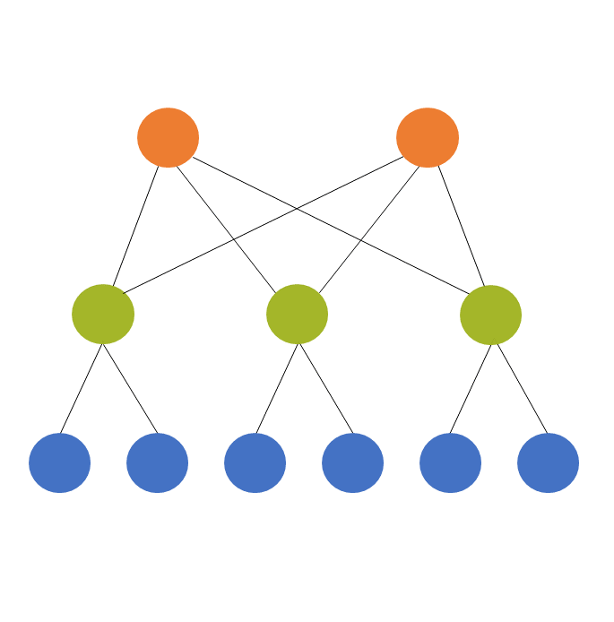
We always count these levels from the bottom up. So if we have students clustered within classroom and classroom clustered within school and school clustered within district, we have:

• Level 1: Students
• Level 2: Classroom
• Level 3: School
• Level 4: District

So this use of the term level describes the design of the study, not the measurement of the variables or the categories of the factors.

Putting them together

So this is the truly unfortunate part. There are situations where all three definitions of level are relevant within the same statistical analysis context.

I find this unfortunate because I think using the same word to mean completely different things just confuses people. But here it is:

Picture that study in which students are clustered within school (a two-level design). Each school is assigned to use one of three math curricula (the independent variable, which happens to be categorical).

So, the variable “math curriculum” is a factor with three levels (ie, three categories).

Because those three categories of “math curriculum” are unordered, “math curriculum” has a nominal level of measurement.

And since “math curriculum” is assigned to each school, it is considered a level 2 variable in the two-level model.

See the rest of the Confusing Statistical Terms series.

First published December 12, 2008

Last Updated January 21, 2025

2 comments