The most basic experimental design is the completely randomized design. It is simple and straightforward when plenty of unrelated subjects are available for an experiment. It’s so simple, it almost seems obvious. But there are important principles in this simple design that are important for tackling more complex experimental designs.
Let’s take a look.
How It Works
The basic idea of any experiment is to learn how different conditions or versions of a treatment affect an outcome. To do this, you assign subjects to different treatment groups. You then run the experiment and record the results for each subject.
Afterward, you use statistical methods to determine whether the different treatment groups have different outcomes.
Key principles for any experimental design are randomization, replication, and reduction of variance. Randomization means assigning the subjects to the different groups in a random way.
Replication means ensuring there are multiple subjects in each group.
Reduction of variance refers to removing or accounting for systematic differences among subjects. Completely randomized designs address the first two principles in a simple way.
To execute a completely randomized design, first determine how many versions of the treatment there are. Next determine how many subjects are available. Divide the number of subjects by the number of treatments to get the number of subjects in each group.
The final design step is to randomly assign individual subjects to fill the spots in each group.
Example
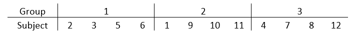
Suppose you are running an experiment. You want to compare three training regimens that may affect the time it takes to run one mile. You also have 12 human subjects who are willing to participate in the experiment. Because you have three training regimens, you will have 12/3 = 4 subjects in each group.
Statistical software (or even Excel) can do the actual assignment. You only need to start by numbering the subjects from 1 to 12 in any way that is convenient. The following table shows one possible random assignment of 12 subjects to three groups.
It’s okay if the number of replicates in each group isn’t exactly the same. Make them as even as possible and assign more to groups that are more interesting to you. Modern statistical software has no trouble adjusting for different sample sizes.
When there is more than one treatment variable, not much changes. Use the combination of treatments when performing random assignment.
For example, say that you add a diet treatment with two conditions in addition to the training. Combined with the three versions of training, there are six possible treatment groups. Assign the subjects in the exact way already described, but with six groups instead of three.
Do not skip randomization! Randomization is the only way to ensure your groups are similar except for the treatment. This is important to ensuring you can attribute group differences to the treatment.
When This Design DOESN’T Work
The completely randomized design is excellent when plenty of unrelated subjects are available to sample. But some situations call for more advanced designs.
This design doesn’t address the third principle of experimental design, reduction of variance.
Sure, you may be able to address this by adding covariates to the analysis. These are variables that are not experimentally assigned but you can measure them. But if reduction of variance is important, other designs do this better.
If some of the subjects are related to each other or a single subject is exposed to multiple conditions of a treatment, you’re going to need another design.
Sometimes it is important to measure outcomes more than once during experimental treatment. For example, you might want to know how quickly the subjects make progress in their training. Again, any repeated measures of outcomes constitute a more complicated design.
Strengths of the Completely Randomized Design
When it works, it has many strengths.
It’s not only easy to create, it’s straightforward to analyze. The results are relatively easy to explain to a non-statistical audience.
Finally, familiarity with this design will help you recognize when it isn’t appropriate. Understanding the ways in which it is not appropriate can help you choose a more advanced design.
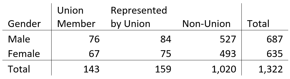
A chi square test is often applied to two-way tables, like the one below.
This table represents a sample of 1,322 individuals. Of these individuals, 687 are male, and 635 are female. Also 143 are union members, 159 are represented by unions, and 1,020 are not affiliated with a union.
You might use a chi-square test if you want to learn something about the relationship of gender and union status. The question then might come up: should you use a test of independence, or a test of homogeneity?
Does it matter? Software doesn’t generally differentiate between the two, which leads to a final question: are they even different?
Well, yes and no. Read on!
Different: Independence versus Homogeneity
Independence and homogeneity do refer to different ideas. If union status and gender are independent, that means that union status and gender are unrelated. In other words, if you know someone’s union status, you won’t be able to make a better guess as to their gender.
If you know someone’s gender, you won’t be able to make a better guess as to their union status.
Homogeneity is different and refers to the concept of similarity. If you are familiar with linear regression, you might associate this with residuals. Residuals should be homogeneous, meaning they all come from the same distribution.
That idea applies to this two-way table as well. We may want to know if the distribution of union status is the same for men and women. In other words, does union status come from the same distribution for both men and women?
To test independence, we would not approach the question from the standpoint of gender or union status. We would take a sample of all employed individuals, and then break them down into the categories in the table.
To test homogeneity, we would approach it from the standpoint of gender. We would randomly sample individuals from within each gender, and then measure their union status.
Either approach would result in the table above.
Same: Chi-Square Statistics
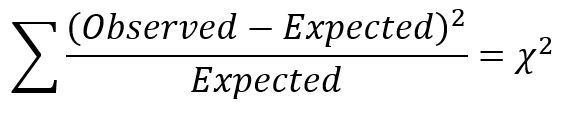
Chi-square statistics for categorical data generally follow this formula:
For each of the six cells representing a combination of gender and union status, the number in the cell is the count we observe. “Expected” refers to what we would see in each cell under the null hypothesis. That means if gender and union status are independent (or if union status is homogeneous across the genders).
We calculate the difference, square it, and divide by the expected count for each cell. We then add these all together, and that is the chi-square test statistic.
Where do we get the expected counts for each cell?
Let’s examine the combination of male and union member under independence. If gender and union membership are independent, then how many male union members do we expect? Well,
– 10.81% of the sample are union members
– 51.96% are male
So, if they are independent, 10.81% x 51.96% is 5.62%, and 5.62% of 1,322 is 74.3. This is how many individuals we would expect to be male union members.
Now let’s consider male union members under homogeneity. Overall, 10.81% of the sample are union members. If this is the same for both males and females, then of the 687 males, we expect 74.3 to be union members.
Independence and homogeneity result in the same expected number of union members! It turns out this calculation is the same for every cell in the table. It follows that the chi-square statistic is also the same.
Does It Matter?
As it turns out, independence and homogeneity are two sides of the same coin. If gender and union status are independent, then union status is distributed the same way for males and females.
So which test should you say you are using, if they turn out the same?
Again, that comes back to how you have phrased your research question. Are you determining whether gender and union status are related. That is a test of independence. Are you looking for differences between males and females? That is a test of homogeneity.
If you analyze non-experimental data, is it helpful to understand experimental design principles?
Yes, absolutely! Understanding experimental design can help you recognize the questions you can and can’t answer with the data. It will also help you identify possible sources of bias that can lead to undesirable results. Finally, it will help you provide recommendations to make future studies more efficient. (more…)
Have you ever wondered why there are so many different types of experimental designs, and how a researcher would go about choosing among them to best address their research questions? (more…)
When learning about linear models —that is, regression, ANOVA, and similar techniques—we are taught to calculate an R2. The R2 has the following useful properties:
The range is limited to [0,1], so we can easily judge how relatively large it is.
It is standardized, meaning its value does not depend on the scale of the variables involved in the analysis.
The interpretation is pretty clear: It is the proportion of variability in the outcome that can be explained by the independent variables in the model.
The calculation of the R2 is also intuitive, once you understand the concepts of variance and prediction. (more…)
What are the best methods for checking a generalized linear mixed model (GLMM) for proper fit?
This question comes up frequently.
Unfortunately, it isn’t as straightforward as it is for a general linear model.
In linear models the requirements are easy to outline: linear in the parameters, normally distributed and independent residuals, and homogeneity of variance (that is, similar variance at all values of all predictors).
The Analysis Factor uses cookies to ensure that we give you the best experience of our website. If you continue we assume that you consent to receive cookies on all websites from The Analysis Factor.
This website uses cookies to improve your experience while you navigate through the website. Out of these, the cookies that are categorized as necessary are stored on your browser as they are essential for the working of basic functionalities of the website. We also use third-party cookies that help us analyze and understand how you use this website. These cookies will be stored in your browser only with your consent. You also have the option to opt-out of these cookies. But opting out of some of these cookies may affect your browsing experience.
Necessary cookies are absolutely essential for the website to function properly. This category only includes cookies that ensures basic functionalities and security features of the website. These cookies do not store any personal information.
Any cookies that may not be particularly necessary for the website to function and is used specifically to collect user personal data via analytics, ads, other embedded contents are termed as non-necessary cookies. It is mandatory to procure user consent prior to running these cookies on your website.
 The most basic experimental design is the completely randomized design. It is simple and straightforward when plenty of unrelated subjects are available for an experiment. It’s so simple, it almost seems obvious. But there are important principles in this simple design that are important for tackling more complex experimental designs.