Ordinary Least Squares regression provides linear models of continuous variables. However, much data of interest to statisticians and researchers are not continuous and so other methods must be used to create useful predictive models.
The glm() command is designed to perform generalized linear models (regressions) on binary outcome data, count data, probability data, proportion data and many other data types.
In this blog post, we explore the use of R’s glm() command on one such data type. Let’s take a look at a simple example where we model binary data.
(more…)
Need to run a logistic regression in SPSS? Turns out, SPSS has a number of procedures for running different types of logistic regression.
Some types of logistic regression can be run in more than one procedure. For some unknown reason, some procedures produce output others don’t. So it’s helpful to be able to use more than one.
Logistic Regression
 Logistic Regression can be used only for binary dependent (more…)
One of the most confusing things about statistical analysis is the different vocabulary used for the same, or nearly-but-not-quite-the-same, concepts.

Sometimes this happens just because the same analysis was developed separately within different fields and named twice.
So people in different fields use different terms for the same statistical concept. Try to collaborate with a colleague in a different field and you may find yourself awed by the crazy statistics they’re insisting on.
Other times, there is a level of detail that is implied by one term that isn’t true of the wider, more generic term. This level of detail is often about how the role of variables or effects affects the interpretation of output. (more…)
Multicollinearity isn’t an assumption of regression models; it’s a data issue.
And while it can be seriously problematic, more often it’s just a nuisance.
In this webinar, we’ll discuss:
- What multicollinearity is and isn’t
- What it does to your model and estimates
- How to detect it
- What to do about it, depending on how serious it is
Note: This training is an exclusive benefit to members of the Statistically Speaking Membership Program and part of the Stat’s Amore Trainings Series. Each Stat’s Amore Training is approximately 90 minutes long.
(more…)
In a statistical model–any statistical model–there is generally one way that a predictor X and a response Y can relate:
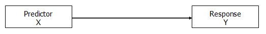
This relationship can take on different forms, of course, like a line or a curve, but there’s really only one relationship here to measure.
Usually the point is to model the predictive or explanatory ability, the effect, of X on Y.
In other words, there is a clear response variable*, although not necessarily a causal relationship. We could have switched the direction of the arrow to indicate that Y predicts X. Or used a two-headed arrow to show a correlation, with no direction, but that’s a whole other story.
For our purposes, Y is the response variable and X the predictor.
But a third variable–another predictor–can relate to X and Y in a number of different ways. How this predictor relates to X and Y changes how we interpret the relationship between X and Y. (more…)
What is the relationship between predictors and whether and when an event will occur?
This is what event history (a.k.a., survival) analysis tests.
There are many flavors of Event History Analysis, though, depending on how time is measured, whether events can repeat, etc.
In this webinar, we discussed many of the issues involved in measuring time, including censoring, and introduce one specific type of event history model: the logistic model for discrete time events.
Note: This training is an exclusive benefit to members of the Statistically Speaking Membership Program and part of the Stat’s Amore Trainings Series. Each Stat’s Amore Training is approximately 90 minutes long.
(more…)