Five Common Relationships Among Three Variables in a Statistical Model

In a statistical model–any statistical model–there is generally one way that a predictor X and a response Y can relate:

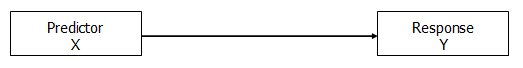
This relationship can take on different forms, of course, like a line or a curve, but there’s really only one relationship here to measure.

Usually the point is to model the predictive ability, the effect, of X on Y.

In other words, there is a clear response variable*, although not necessarily a causal relationship. We could have switched the direction of the arrow to indicate that Y predicts X or used a two-headed arrow to show a correlation, with no direction, but that’s a whole other story.

For our purposes, Y is the response variable and X the predictor.

But a third variable–another predictor–can relate to X and Y in a number of different ways.  How this predictor relates to X and Y changes how we interpret the relationship between X and Y.These relationships have common names, but the names sometimes differ across fields, so you may be familiar with a different name than the ones I give below.  In any case, the names are less important than:

1. making sure the relationship you are testing is the one that answers your research question and

2. the relationship reflects the data.

So let’s look at some possible relationships, once we add a second predictor, Z.

1. Covariate correlated with X

In this model, the Covariate, Z,  is correlated with X, and both predict Y.

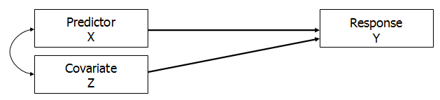
Because X and Z are not independent, there will usually be some joint effect on Y–some part of the relationship between X and Y that can’t be distinguished from the relationship between Z and Y.

The relationship between X and Y is no longer the full effect of X on Y.

It’s the marginal, unique effect of X on Y, after controlling for the effect of Z.

While the model fit as a whole will include both the joint and the unique effects of both X and Z on Y, the regression coefficient for X will only include its unique effect.

When both X and Z are observed variables, this is nearly always the situation.

As long as the correlation is moderate, it’s still possible to measure the unique effect of X.  If it gets too high, however, you will start to hit a point of multicollinearity in which the model has problems calculating estimates.

A good example of this kind of relationship would be in a study that measures the nutritional composition of soil cores at different altitudes and moisture levels.

Because water flows downhill, lower altitudes (X) tend to be more moist (Z). So while we can’t completely separate altitude from moisture levels, as long as they’re only moderately correlated, we should be able to find the unique effect of altitude on potassium levels.

Test this effect by including X and Z in a model together.  To understand how much Z and X overlap in their explanation of Y, rerun the model without Z and look at how much X’s coefficient changes.

2. Covariate Independent of X

When a covariate Z  is NOT related to X, it has a slightly different effect.  It needs to be able to predict Y as well to be useful in the model, but the effects of X and Z don’t overlap.

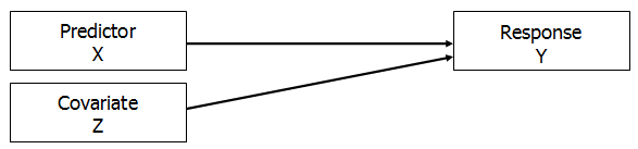
Including Z in the model often leads to the relationship between X and Y becoming more significant because Z has explained some of the otherwise unexplained variance in Y.

An example of this kind of covariate is when an experimental manipulation (X) on response time (Y) only becomes significant when we control for finger dexterity levels (Z).

If finger dexterity has a large effect on response time and we don’t account for it, all of that variation due to dexterity will go into unexplained error–the denominator of our test statistic.

Controlling for that variance means it is no longer unexplained, and is removed from the denominator.

Test this type of effect by running hierarchical regression (add each predictor in on a separate step).

3. Spurious Relationship

A confounding variable Z creates a spurious relationship between X and Y because Z is related to both X and Y.

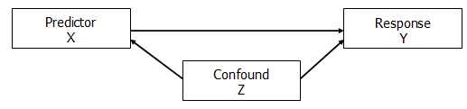
This is the relationship seen in most “correlation is not causation” examples: The amount of ice cream consumption (X) in  a month predicts number of shark attacks (Y). Do sharks like eating ice-cream laden people?  No.

This spurious relationship is created by a confounder that leads to increases in both ice-cream consumption and shark attacks: temperature (Z). People both eat more ice cream and swim in the ocean in hotter months.

It can be difficult to distinguish between this relationship and #1 above through testing alone.  This is a situation where you have to entertain spuriousness as a possibility and question your results.

4. Mediation

Mediation indicates a specific causal pathway.  It occurs when at least part of the reason X affects Y is through Z.  X affects Z and Z affects Y.

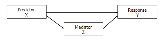
There are then two effects of X on Y: the indirect effect of X on Y through Z and the direct effect of X on Y.

An example here would be if the relationship between stress (X) and depression (Y) was mediated through increased levels of stress hormones (Z).

There are a number of ways to test for mediation, including running a series of regression models and through path analysis.  More modern approaches recommend testing the strength of the indirect effect.

5. Moderation

Despite the similarity in the names, a moderation is an entirely different beast than mediation.

Moderation indicates that the effect of X on Y is different for different values of Z.  In other words, Z moderates (affects) the effect of X on Y.

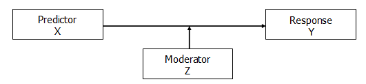
Maybe when Z is large, there is a strong positive relationship between X and Y, but when Z is small, there is no relationship between X and Y.

So essentially, we’re saying that X predicts Y in different ways, depending on the value of Z.

X and Z can be correlated or not.

One example of moderation can be seen in the relationship between depression (X), physical health scores (Y), and poverty status (Z).  Poverty status (Yes/No) would be said to moderate  the relationship between depression and physical health if there was a weak negative relationship among people not in poverty, but a strong negative relationship among people in poverty.

Test moderation by including an interaction term between X and Z.

All of these relationships can occur with more than two predictors in the model, and a model can contain more than one of them.  Figuring out the potential relationships among variables is often the fun part of data analysis.

Four Critical Steps in Building Linear Regression Models

While you’re worrying about which predictors to enter, you might be missing issues that have a big impact your analysis. This training will help you achieve more accurate results and a less-frustrating model building experience.

Take Me to The Video!