Are you learning Multilevel Models? Do you feel ready? Or in over your head?
It’s a very common analysis to need to use. I have to say, learning it is not so easy on your own. The concepts of random effects are hard to wrap your head around and there is a ton of new vocabulary and notation. Sadly, this vocabulary and notation is not consistent across articles, books, and software, so you end up having to do a lot of translating.
(more…)
 If you have a categorical predictor variable that you plan to use in a regression analysis in SPSS, there are a couple ways to do it.
You can use the SPSS Regression procedure. Or you can use SPSS General Linear Model–>Univariate, which I discuss here. If you use Syntax, it’s the UNIANOVA command.
The big question in SPSS GLM is what goes where. As I’ve detailed in another post, any continuous independent variable goes into covariates. And don’t use random factors at all unless you really know what you’re doing.
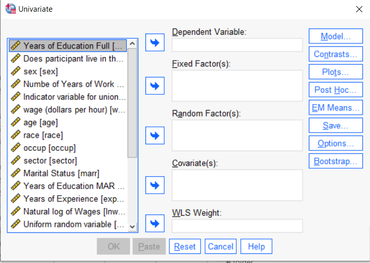
So the question is what to do with your categorical variables. You have two choices, and each has advantages and disadvantages.
The easiest is to put categorical variables in Fixed Factors. SPSS GLM will dummy code those variables for you, which is quite convenient if your categorical variable has more than two categories.
However, there are some defaults you need to be aware of that may or may not make this a good choice.
The dummy coding reference group default
SPSS GLM always makes the reference group the one that comes last alphabetically.
So if the values you input are strings, it will be the one that comes last. If those values are numbers, it will be the highest one.
Not all procedures in SPSS use this default so double check the default if you’re using something else. Some procedures in SPSS let you change the default, but GLM doesn’t.
In some studies it really doesn’t matter which is the reference group.
But in others, interpreting regression coefficients will be a whole lot easier if you choose a group that makes a good comparison such as a control group or the most common group in the data.
If you want that to be the reference group in SPSS GLM, make it come last alphabetically. I’ve been known to do things like change my data so that the control group becomes something like ZControl. (But create a new variable–never overwrite original data).
It really can get confusing, though, if the variable was already dummy coded–if it already had values of 0 and 1. Because 1 comes last alphabetically, SPSS GLM will make that group the reference group and internally code it as 0.
This can really lead to confusion when interpreting coefficients. It’s not impossible if you’re paying attention, but you do have to pay attention. It’s generally better to recode the variable so that you don’t confuse yourself. And while you may believe you’re up for overcoming the confusion, why make things harder on yourself or with any other colleague you’re sharing results with?
Interactions among fixed factors default
There is another key default to keep in mind. GLM will automatically create interactions between any and all variables you specify as Fixed Factors.
If you put 5 variables in Fixed Factors, you’ll get a lot of interactions. SPSS will automatically create all 2-way, 3-way, 4-way, and even a 5-way interaction among those 5 variables.
That’s a lot of interactions.
In contrast, GLM doesn’t create by default any interactions between Covariates or between Covariates and Fixed Factors.
So you may find you have more interactions than you wanted among your categorical predictors. And fewer interactions than you wanted among numerical predictors.
There is no reason to use the default. You can override it quite easily.
Just click on the Model button. Then choose “Custom Model.” You can then choose which interactions you do, or don’t, want in the model.
If you’re using SPSS syntax, simply add the interactions you want to the /Design subcommand.
So think about which interactions you want in the model. And take a look at whether your variables are already dummy coded.
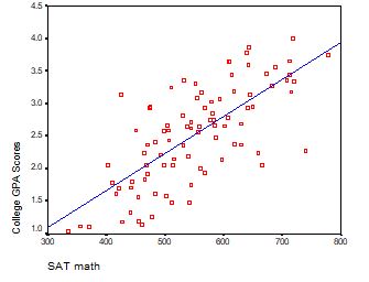
Interpreting the Intercept in a regression model isn’t always as straightforward as it looks.
Here’s the definition: the intercept (often labeled the constant) is the expected value of Y when all X=0. But that definition isn’t always helpful. So what does it really mean?
Regression with One Predictor X
Start with a very simple regression equation, with one predictor, X.
If X sometimes equals 0, the intercept is simply the expected value of Y at that value. In other words, it’s the mean of Y at one value of X. That’s meaningful.
If X never equals 0, then the intercept has no intrinsic meaning. You literally can’t interpret it. That’s actually fine, though. You still need that intercept to give you unbiased estimates of the slope and to calculate accurate predicted values. So while the intercept has a purpose, it’s not meaningful.
Both these scenarios are common in real data. (more…)
Multicollinearity in regression is one of those issues that strikes fear into the hearts of researchers. You’ve heard about its dangers in statistics
classes, and colleagues and journal reviews question your results because of it. But there are really only a few causes of multicollinearity. Let’s explore them.
Multicollinearity is simply redundancy in the information contained in predictor variables. If the redundancy is moderate,
(more…)
Updated 12/20/2021
Despite its popularity, interpreting regression coefficients of any but the simplest models is sometimes, well….difficult.
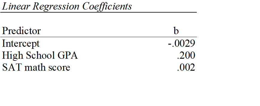
So let’s interpret the coefficients in a model with two predictors: a continuous and a categorical variable. The example here is a linear regression model. But this works the same way for interpreting coefficients from any regression model without interactions.
A linear regression model with two predictor variables results in the following equation:
Yi = B0 + B1*X1i + B2*X2i + ei.
The variables in the model are:
- Y, the response variable;
- X1, the first predictor variable;
- X2, the second predictor variable; and
- e, the residual error, which is an unmeasured variable.
The parameters in the model are:
- B0, the Y-intercept;
- B1, the first regression coefficient; and
- B2, the second regression coefficient.
One example would be a model of the height of a shrub (Y) based on the amount of bacteria in the soil (X1) and whether the plant is located in partial or full sun (X2).
Height is measured in cm. Bacteria is measured in thousand per ml of soil. And type of sun = 0 if the plant is in partial sun and type of sun = 1 if the plant is in full sun.
Let’s say it turned out that the regression equation was estimated as follows:
Y = 42 + 2.3*X1 + 11*X2
Interpreting the Intercept
B0, the Y-intercept, can be interpreted as the value you would predict for Y if both X1 = 0 and X2 = 0.
We would expect an average height of 42 cm for shrubs in partial sun with no bacteria in the soil. However, this is only a meaningful interpretation if it is reasonable that both X1 and X2 can be 0, and if the data set actually included values for X1 and X2 that were near 0.
If neither of these conditions are true, then B0 really has no meaningful interpretation. It just anchors the regression line in the right place. In our case, it is easy to see that X2 sometimes is 0, but if X1, our bacteria level, never comes close to 0, then our intercept has no real interpretation.
Interpreting Coefficients of Continuous Predictor Variables
Since X1 is a continuous variable, B1 represents the difference in the predicted value of Y for each one-unit difference in X1, if X2 remains constant.
This means that if X1 differed by one unit (and X2 did not differ) Y will differ by B1 units, on average.
In our example, shrubs with a 5000/ml bacteria count would, on average, be 2.3 cm taller than those with a 4000/ml bacteria count. They likewise would be about 2.3 cm taller than those with 3000/ml bacteria, as long as they were in the same type of sun.
(Don’t forget that since the measurement unit for bacteria count is 1000 per ml of soil, 1000 bacteria represent one unit of X1).
Interpreting Coefficients of Categorical Predictor Variables
Similarly, B2 is interpreted as the difference in the predicted value in Y for each one-unit difference in X2 if X1 remains constant. However, since X2 is a categorical variable coded as 0 or 1, a one unit difference represents switching from one category to the other.
B2 is then the average difference in Y between the category for which X2 = 0 (the reference group) and the category for which X2 = 1 (the comparison group).
So compared to shrubs that were in partial sun, we would expect shrubs in full sun to be 11 cm taller, on average, at the same level of soil bacteria.
Interpreting Coefficients when Predictor Variables are Correlated
Don’t forget that each coefficient is influenced by the other variables in a regression model. Because predictor variables are nearly always associated, two or more variables may explain some of the same variation in Y.
Therefore, each coefficient does not measure the total effect on Y of its corresponding variable. It would if it were the only predictor variable in the model. Or if the predictors were independent of each other.
Rather, each coefficient represents the additional effect of adding that variable to the model, if the effects of all other variables in the model are already accounted for.
This means that adding or removing variables from the model will change the coefficients. This is not a problem, as long as you understand why and interpret accordingly.
Interpreting Other Specific Coefficients
I’ve given you the basics here. But interpretation gets a bit trickier for more complicated models, for example, when the model contains quadratic or interaction terms. There are also ways to rescale predictor variables to make interpretation easier.
So here is some more reading about interpreting specific types of coefficients for different types of models: