Centering a Covariate to Improve Interpretability

Centering a covariate –a continuous predictor variable–can make regression coefficients much more interpretable. That’s a big advantage, particularly when you have many coefficients to interpret. Or when you’ve included terms that are tricky to interpret, like interactions or quadratic terms.

For example, say you had one categorical predictor with 4 categories and one continuous covariate, plus an interaction between them.

First, you’ll notice that if you center your covariate at the mean, there is no difference in the ANOVA table (called Tests of Between Subjects Effects in SPSS).  This is the table with Sums of Squares and F statistics.  There may be tiny differences due to rounding, but the results should generally not change.

You can interpret the categorical variable via the regression coefficients. But I usually find it easier to use the estimated marginal means (in SPSS; in SAS, they are called least squares means).  These are the means of Y for each group at the mean value of the covariate.  If you centered your covariate at its mean, there should be no difference whatsoever in the estimated marginal means.

Interpreting the Coefficient of the Centered Variable

The covariate and interaction would be interpreted by looking at the regression coefficients in the Parameter Estimates table.

The B values in this table are the regression coefficients (slopes).  With an interaction in the model, the B value for the covariate is the slope when the categorical variable = 0.

The Parameter Estimates table in SPSS GLM automatically dummy codes your categorical variables.  This means it makes the category that comes last alphabetically = 0 (If you numbered them 1, 2, 3, 4, then 4 comes last alphabetically–you can change this default when you run the GLM).  So the B value for the covariate is the slope of the covariate only for group 4.

The B values listed for the interactions with the other groups are the differences in the slopes between each of those groups and group 4.  The p-values for those B values reflect a set of null hypotheses that their slopes are equal to group 4’s slope. No difference.

Again, these don’t change whether you center the covariate or not.

What do change are the intercepts.  And you have four intercepts (one line for each category).  The B labeled Intercept in the output is the intercept just for the reference category (group 4).  The Bs for the other three groups are the differences in intercepts between group 4 and each of those groups.

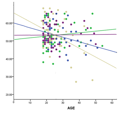
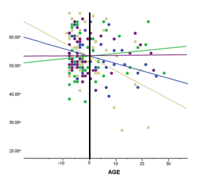Remember the intercept is the mean of the dependent variable when the covariate = 0.  When you center the covariate, you are changing the 0 point.  So the intercepts are no longer the average value when Covariate=0 on its original scale but the average value when the Covariate is at its mean.

This is especially helpful when the Covariate never has values even close to 0.  For example, if your Covariate was Age, and your Ages ranged from 20-60, the mean value of the DV at birth doesn’t make much sense.

First Published 1/27/09;
Updated 4/09/21 to give more detail.

Interpreting Linear Regression Coefficients: A Walk Through Output

Learn the approach for understanding coefficients in that regression as we walk through output of a model that includes numerical and categorical predictors and an interaction.

Take Me to The Video!