March 22nd, 2023 by Karen Grace-Martin
 If you have a categorical predictor variable that you plan to use in a regression analysis in SPSS, there are a couple ways to do it.
You can use the SPSS Regression procedure. Or you can use SPSS General Linear Model–>Univariate, which I discuss here. If you use Syntax, it’s the UNIANOVA command.
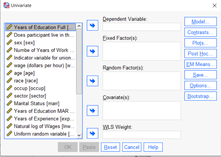
The big question in SPSS GLM is what goes where. As I’ve detailed in another post, any continuous independent variable goes into covariates. And don’t use random factors at all unless you really know what you’re doing.
So the question is what to do with your categorical variables. You have two choices, and each has advantages and disadvantages.
The easiest is to put categorical variables in Fixed Factors. SPSS GLM will dummy code those variables for you, which is quite convenient if your categorical variable has more than two categories.
However, there are some defaults you need to be aware of that may or may not make this a good choice.
The dummy coding reference group default
SPSS GLM always makes the reference group the one that comes last alphabetically.
So if the values you input are strings, it will be the one that comes last. If those values are numbers, it will be the highest one.
Not all procedures in SPSS use this default so double check the default if you’re using something else. Some procedures in SPSS let you change the default, but GLM doesn’t.
In some studies it really doesn’t matter which is the reference group.
But in others, interpreting regression coefficients will be a whole lot easier if you choose a group that makes a good comparison such as a control group or the most common group in the data.
If you want that to be the reference group in SPSS GLM, make it come last alphabetically. I’ve been known to do things like change my data so that the control group becomes something like ZControl. (But create a new variable–never overwrite original data).
It really can get confusing, though, if the variable was already dummy coded–if it already had values of 0 and 1. Because 1 comes last alphabetically, SPSS GLM will make that group the reference group and internally code it as 0.
This can really lead to confusion when interpreting coefficients. It’s not impossible if you’re paying attention, but you do have to pay attention. It’s generally better to recode the variable so that you don’t confuse yourself. And while you may believe you’re up for overcoming the confusion, why make things harder on yourself or with any other colleague you’re sharing results with?
Interactions among fixed factors default
There is another key default to keep in mind. GLM will automatically create interactions between any and all variables you specify as Fixed Factors.
If you put 5 variables in Fixed Factors, you’ll get a lot of interactions. SPSS will automatically create all 2-way, 3-way, 4-way, and even a 5-way interaction among those 5 variables.
That’s a lot of interactions.
In contrast, GLM doesn’t create by default any interactions between Covariates or between Covariates and Fixed Factors.
So you may find you have more interactions than you wanted among your categorical predictors. And fewer interactions than you wanted among numerical predictors.
There is no reason to use the default. You can override it quite easily.
Just click on the Model button. Then choose “Custom Model.” You can then choose which interactions you do, or don’t, want in the model.
If you’re using SPSS syntax, simply add the interactions you want to the /Design subcommand.
So think about which interactions you want in the model. And take a look at whether your variables are already dummy coded.
August 18th, 2021 by Karen Grace-Martin
Updated 8/18/2021
I recently was asked whether to report means from descriptive statistics or from the Estimated Marginal Means with SPSS GLM.
The short answer: Report the Estimated Marginal Means (almost always).
To understand why and the rare case it doesn’t matter, let’s dig in a bit with a longer answer.
First, a marginal mean is the mean response for each category of a factor, adjusted for any other variables in the model (more on this later).
Just about any time you include a factor in a linear model, you’ll want to report the mean for each group. The F test of the model in the ANOVA table will give you a p-value for the null hypothesis that those means are equal. And that’s important.
But you need to see the means and their standard errors to interpret the results. The difference in those means is what measures the effect of the factor. While that difference can also appear in the regression coefficients, looking at the means themselves give you a context and makes interpretation more straightforward. This is especially true if you have interactions in the model.
Some basic info about marginal means
- In SPSS menus, they are in the Options button and in SPSS’s syntax they’re EMMEANS.
- These are called LSMeans in SAS, margins in Stata, and emmeans in R’s emmeans package.
- Although I’m talking about them in the context of linear models, all the software has them in other types of models, including linear mixed models, generalized linear models, and generalized linear mixed models.
- They are also called predicted means, and model-based means. There are probably a few other names for them, because that’s what happens in statistics.
When marginal means are the same as observed means
Let’s consider a few different models. In all of these, our factor of interest, X, is a categorical predictor for which we’re calculating Estimated Marginal Means. We’ll call it the Independent Variable (IV).
Model 1: No other predictors
If you have just a single factor in the model (a one-way anova), marginal means and observed means will be the same.
Observed means are what you would get if you simply calculated the mean of Y for each group of X.
Model 2: Other categorical predictors, and all are balanced
Likewise, if you have other factors in the model, if all those factors are balanced, the estimated marginal means will be the same as the observed means you got from descriptive statistics.
Model 3: Other categorical predictors, unbalanced
Now things change. The marginal mean for our IV is different from the observed mean. It’s the mean for each group of the IV, averaged across the groups for the other factor.
When you’re observing the category an individual is in, you will pretty much never get balanced data. Even when you’re doing random assignment, balanced groups can be hard to achieve.
In this situation, the observed means will be different than the marginal means. So report the marginal means. They better reflect the main effect of your IV—the effect of that IV, averaged across the groups of the other factor.
Model 4: A continuous covariate
When you have a covariate in the model the estimated marginal means will be adjusted for the covariate. Again, they’ll differ from observed means.
It works a little bit differently than it does with a factor. For a covariate, the estimated marginal mean is the mean of Y for each group of the IV at one specific value of the covariate.
By default in most software, this one specific value is the mean of the covariate. Therefore, you interpret the estimated marginal means of your IV as the mean of each group at the mean of the covariate.
This, of course, is the reason for including the covariate in the model–you want to see if your factor still has an effect, beyond the effect of the covariate. You are interested in the adjusted effects in both the overall F-test and in the means.
If you just use observed means and there was any association between the covariate and your IV, some of that mean difference would be driven by the covariate.
For example, say your IV is the type of math curriculum taught to first graders. There are two types. And say your covariate is child’s age, which is related to the outcome: math score.
It turns out that curriculum A has slightly older kids and a higher mean math score than curriculum B. Observed means for each curriculum will not account for the fact that the kids who received that curriculum were a little older. Marginal means will give you the mean math score for each group at the same age. In essence, it sets Age at a constant value before calculating the mean for each curriculum. This gives you a fairer comparison between the two curricula.
But there is another advantage here. Although the default value of the covariate is its mean, you can change this default. This is especially helpful for interpreting interactions, where you can see the means for each group of the IV at both high and low values of the covariate.
In SPSS, you can change this default using syntax, but not through the menus.
For example, in this syntax, the EMMEANS statement reports the marginal means of Y at each level of the categorical variable X at the mean of the Covariate V.
UNIANOVA Y BY X WITH V
/INTERCEPT=INCLUDE
/EMMEANS=TABLES(X) WITH(V=MEAN)
/DESIGN=X V.
If instead, you wanted to evaluate the effect of X at a specific value of V, say 50, you can just change the EMMEANS statement to:
/EMMEANS=TABLES(X) WITH(V=50)
Another good reason to use syntax.
April 9th, 2021 by Karen Grace-Martin
Centering a covariate –a continuous predictor variable–can make regression coefficients much more interpretable. That’s a big advantage, particularly when you have many coefficients to interpret. Or when you’ve included terms that are tricky to interpret, like interactions or quadratic terms.
For example, say you had one categorical predictor with 4 categories and one continuous covariate, plus an interaction between them.
First, you’ll notice that if you center your covariate at the mean, there is (more…)
December 3rd, 2009 by Karen Grace-Martin
One of the biggest challenges in learning statistics and data analysis is learning the lingo. It doesn’t help that half of the notation is in Greek (literally).
The terminology in statistics is particularly confusing because often the same word or symbol is used to mean completely different concepts.
I know it feels that way, but it really isn’t a master plot by statisticians to keep researchers feeling ignorant.
Really.
It’s just that a lot of the methods in statistics were created by statisticians working in different fields–economics, psychology, medicine, and yes, straight statistics. Certain fields often have specific types of data that come up a lot and that require specific statistical methodologies to analyze.
Economics needs time series, psychology needs factor analysis. Et cetera, et cetera.
But separate fields developing statistics in isolation has some ugly effects.
Sometimes different fields develop the same technique, but use different names or notation.
Other times different fields use the same name or notation on different techniques they developed.
And of course, there are those terms with slightly different names, often used in similar contexts, but with different meanings. These are never used interchangeably, but they’re easy to confuse if you don’t use this stuff every day.
And sometimes, there are different terms for subtly different concepts, but people use them interchangeably. (I am guilty of this myself). It’s not a big deal if you understand those subtle differences. But if you don’t, it’s a mess.
And it’s not just fields–it’s software, too.
SPSS uses different names for the exact same thing in different procedures. In GLM, a continuous independent variable is called a Covariate. In Regression, it’s called an Independent Variable.
Likewise, SAS has a Repeated statement in its GLM, Genmod, and Mixed procedures. They all get at the same concept there (repeated measures), but they deal with it in drastically different ways.
So once the fields come together and realize they’re all doing the same thing, people in different fields or using different software procedures, are already used to using their terminology. So we’re stuck with different versions of the same word or method.
So anyway, I am beginning a series of blog posts to help clear this up. Hopefully it will be a good reference you can come back to when you get stuck.
We’ve expanded on this list with a member training, if you’re interested.
If you have good examples, please post them in the comments. I’ll do my best to clear things up.
October 30th, 2009 by Karen Grace-Martin
Maybe I’ve noticed it more because I’m getting ready for next week’s SPSS in GLM workshop. Just this week, I’ve had a number of experiences with people’s struggle with SPSS, and GLM in particular.
Number 1: I read this in a technical report by Patrick Burns comparing SPSS to R:
“SPSS is notorious for its attitude of ‘You want to do one of these things. If you don’t understand what the output means, click help and we’ll pop up five lines of mumbo-jumbo that you’re not going to understand either.’ “
And while I still prefer SPSS, I had to laugh because the anonymous person Burns (more…)
October 7th, 2009 by Karen Grace-Martin
You don’t rely on only SPSS menus to run your analysis, right? (Please, please tell me you don’t).
There’s really nothing wrong with using the menus. It’s a great way to get started using SPSS and it saves you the hassle of remembering all that code.
But there are some really, really good reasons to use the syntax as well.
1. Efficiency
If you’re figuring out the best model and have to refine which predictors to include, running the same descriptive statistics on a bunch of variables, or defining the missing values for all 286 variable in the data set, you’re essentially running the same analysis over and over.
Picking your way through the menus gets old fast. In syntax, you just copy and paste and change or add variables names.
A trick I use is to run through the menus for one variable, paste the code, then add the other 285. You can even copy the names out of the Variable View and paste them into the code. Very easy.
2. Memory
I know that while you’re immersed in your data analysis, you can’t imagine you won’t always remember every step you did.
But you will. And sooner than you think.
Syntax gives you a “paper” trail of what you did, so you don’t have to remember. If you’re in a regulated industry, you know why you need this trail. But anyone who needs to defend their research needs it.
3. Communication
When your advisor, coauthor, colleague, statistical consultant, or Reviewer #2 asks you which options you used in your analysis or exactly how you recoded that variable, you can clearly communicate it by showing the syntax. Much harder to explain with menu options.
When I hold a workshop or run an analysis for a client, I always use syntax. I send it to them to peruse, tweak, adapt, or admire. It’s really the only way for me to show them exactly what I did and how to do it.
If your client, advisor, or colleague doesn’t know how to read the syntax, that’s okay. Because you have a clear answer of what you did, you can explain it.
4. Efficiency again
When the data set gets updated, or a reviewer (or your advisor, coauthor, colleague, or statistical consultant) asks you to add another predictor to a model, it’s a simple matter to edit and rerun a syntax program.
In menus, you have to start all over. Hopefully you’ll remember exactly which options you chose last time and/or exactly how you made every small decision in your data analysis (see #2: Memory).
5. Control
There are some SPSS options that are available in syntax, but not in the menus.
And others that just aren’t what they seem in the menus.
The menus for the Mixed procedure are about the most unintuitive I’ve ever seen. But the syntax for Mixed is really logical and straightforward. And it’s very much like the GLM syntax (UNIANOVA), so if you’re familiar with GLM, learning Mixed is a simple extension.
Bonus Reason to use SPSS Syntax: Cleanliness
Luckily, SPSS makes it exceedingly easy to create syntax. If you’re more comfortable with menus, run it in menus the first time, then hit PASTE instead of OK. SPSS will automatically create the syntax for you, which you can alter at will. So you don’t have to remember every programming convention.
When refining a model, I often run through menus and paste it. Then I alter the syntax to find the best-fitting model.
At this point, the output is a mess, filled with so many models I can barely keep them straight. Once I’ve figured out the model that fits best, I delete the entire output, then rerun the syntax for only the best model. Nice, clean output.
The Take-away: Reproducibility
What this all really comes down to is your ability to confidently, easily, and accurately reproduce your analysis. When you rely on menus, you are relying on your own memory to reproduce. There are too many decisions, judgments, and too many places to make easy mistakes without noticing it to ever be able to rely totally on your memory.
The tools are there to make this easy. Use them.