When we run a statistical model, we are in a sense creating a mathematical equation. The simplest regression model looks like this:
Yi = β0 + β1X+ εi
The left side of the equation is the sum of two parts on the right: the fixed component, β0 + β1X, and the random component, εi.
You’ll also sometimes see the equation written (more…)
Generalized linear models—and generalized linear mixed models—are called generalized linear because they connect a model’s outcome to its predictors in a linear way. The function used to make this connection is called a link function. Link functions sounds like an exotic term, but they’re actually much simpler than they sound.
For example, Poisson regression (commonly used for outcomes that are counts) makes use of a natural log link function as follows:
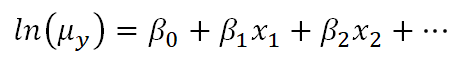
Clearly, there is not a direct linear relationship of the x variables to the average count, but there is a “sort of linear” relationship happening: a function of the mean of y is related to a linear combination of x variables. In other words, the linear model has now been generalized to a bigger type of situation.
This can lead to confusion, though, because on the surface it looks very similar to what happens when we transform the dependent variable in a linear model, like a linear regression.
The key thing to understand is that the natural log link function is a function of the mean of y, not the y values themselves.
Transformations of Y
Below is a linear model equation where the original dependent variable, y, has been natural log transformed. That is, the natural log has been taken of each individual value of y, and that is being used as the dependent variable.
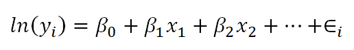
The linear model with the log transformation is providing an equation for an individual value of ln(y). We could also write it as follows, where we are modeling the mean of ln(y) (note the error term is no longer present):
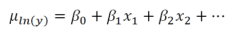
This makes the difference a bit clearer. When we transform the data in a linear model, we are no longer claiming that y is normally distributed around a mean, given the x values — we are claiming that our new outcome variable, ln(yi), is normally distributed.
In fact, we often make this transformation specifically because the values of y do not appear to be normally distributed around their average.
In the case of the Poisson model, however, the link function does not change the distribution of the actual observations in some way to make them something other than Poisson distributed. Instead, the link function defines the relationship of the x variables directly to the mean of the Poisson distributed y. The individual observations then vary around this expected value accordingly.
The mean of the log is not the log of the mean
As you may know, if you have used this kind of data transformation in a linear model before, you cannot simply take the exponent of the mean of ln(y) to get the mean of y.
You might be surprised to know, though, that you can do this with a link function. If you have specific values of your x variables, you can calculate the predicted average count, μy based on those x values by inversing the natural log:
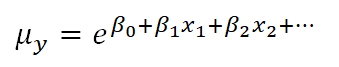
This ability to back-transform means (and regression coefficients) to a more intuitive scale is part of what makes generalized linear models so useful.
Go to the next article or see the full series on Easy-to-Confuse Statistical Concepts
One important yet difficult skill in statistics is choosing a type model for different data situations. One key consideration is the dependent variable.
For linear models, the dependent variable doesn’t have to be normally distributed, but it does have to be continuous, unbounded, and measured on an interval or ratio scale.
Percentages don’t fit these criteria. Yes, they’re continuous and ratio scale. The issue is the (more…)
Imagine this scenario:
This year’s flu strain is very vigorous. The number of people checking in at hospitals is rapidly increasing. Hospitals are desperate to know if they have enough beds to handle those who need their help.
You have been asked to analyze a previous year’s hospitalization length of stay by people with the flu who had been admitted to the hospital. The predictors in your data set are age group, gender and race of those admitted. You also have an indicator that signifies whether the hospital was privately or publicly run.
(more…)
The normal distribution is so ubiquitous in statistics that those of us who use a lot of statistics tend to forget it’s not always so common in actual data.
And since the normal distribution is continuous, many people describe all numerical variables as continuous. I get it: I’m guilty of using those terms interchangeably, too, but they’re not exactly the same.
Numerical variables can be either continuous or discrete.
The difference? Continuous variables can take any number within a range. Discrete variables can only take on specific values. For numeric discrete data, these are often, but don’t have to be, whole numbers*.
Count variables, as the name implies, are frequencies of some event or state. Number of arrests, fish (more…)
