Spearman correlation

Is it really ok to treat Likert items as continuous? 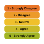And can you just decide to combine Likert items to make a scale? Likert-type data is extremely common—and so are questions like these about how to analyze it appropriately. (more…)

1 comment

What does it mean for two variables to be correlated?

Is that the same or different than if they’re associated or related?

This is the kind of question that can feel silly, but shouldn’t. It’s just a reflection of the confusing terminology used in statistics. In this case, the technical statistical term looks like, but is not exactly the same as, the way we mean it in everyday English. (more…)

9 comments

Let’s use R to explore bivariate relationships among variables.

Part 7 of this series showed how to do a nice bivariate plot, but it’s also useful to have a correlation statistic.

We use a new version of the data set we used in Part 20 of tourists from different nations, their gender, and number of children. Here, we have a new variable – the amount of money they spend while on vacation.

First, if the data object (A) for the previous version of the tourists data set is present in your R workspace, it is a good idea to remove it because it has some of the same variable names as the data set that you are about to read in. We remove A as follows:

rm(A)

Removing the object A ensures no confusion between different data objects that contain variables with similar names.

Now copy and paste the following array into R.

M <- structure(list(COUNTRY = structure(c(3L, 3L, 3L, 3L, 1L, 3L, 2L, 3L, 1L, 3L, 3L, 1L, 2L, 2L, 3L, 3L, 3L, 2L, 3L, 1L, 1L, 3L,
1L, 2L), .Label = c("AUS", "JAPAN", "USA"), class = "factor"),GENDER = structure(c(2L, 1L, 2L, 2L, 1L, 2L, 1L, 2L, 1L, 2L, 2L, 1L, 1L, 1L, 1L, 2L, 1L, 1L, 2L, 2L, 1L, 1L, 1L, 2L), .Label = c("F", "M"), class = "factor"), CHILDREN = c(2L, 1L, 3L, 2L, 2L, 3L, 1L, 0L, 1L, 0L, 1L, 2L, 2L, 1L, 1L, 1L, 0L, 2L, 1L, 2L, 4L, 2L, 5L, 1L), SPEND = c(8500L, 23000L, 4000L, 9800L, 2200L, 4800L, 12300L, 8000L, 7100L, 10000L, 7800L, 7100L, 7900L, 7000L, 14200L, 11000L, 7900L, 2300L, 7000L, 8800L, 7500L, 15300L, 8000L, 7900L)), .Names = c("COUNTRY", "GENDER", "CHILDREN", "SPEND"), class = "data.frame", row.names = c(NA, -24L))


M
attach(M)

Do tourists with greater numbers of children spend more? Let’s calculate the correlation between CHILDREN and SPEND, using the cor() function.

R <- cor(CHILDREN, SPEND)
[1] -0.2612796


We have a weak correlation, but it’s negative! Tourists with a greater number of children tend to spend less rather than more!

(Even so, we’ll plot this in our next post to explore this unexpected finding).

We can round to any number of decimal places using the round() command.

round(R, 2)
[1] -0.26

The percentage of shared variance (100*r²) is:
100 * (R**2)
[1] 6.826704

To test whether your correlation coefficient differs from 0, use the cor.test() command.

cor.test(CHILDREN, SPEND)
Pearson's product-moment correlation
data: CHILDREN and SPEND
t = -1.2696, df = 22, p-value = 0.2175
alternative hypothesis: true correlation is not equal to 0
95 percent confidence interval:
-0.6012997 0.1588609
sample estimates:
cor
-0.2612796

The cor.test() command returns the correlation coefficient, but also gives the p-value for the correlation. In this case, we see that the correlation is not significantly different from 0 (p is approximately 0.22).

Of course we have only a few values of the variable CHILDREN, and this fact will influence the correlation. Just how many values of CHILDREN do we have? Can we use the levels() command directly? (Recall that the term “level” has a few meanings in statistics, once of which is the values of a categorical variable, aka “factor“).

levels(CHILDREN)
NULL

R does not recognize CHILDREN as a factor. In order to use the levels() command, we must turn CHILDREN into a factor temporarily, using as.factor().

levels(as.factor(CHILDREN))
[1] "0" "1" "2" "3" "4" "5"

So we have six levels of CHILDREN. CHILDREN is a discrete variable without many values, so a Spearman correlation can be a better option. Let’s see how to implement a Spearman correlation:

cor(CHILDREN, SPEND, method ="spearman")
[1] -0.3116905

We have obtained a similar but slightly different correlation coefficient estimate because the Spearman correlation is indeed calculated differently than the Pearson.

Why not plot the data? We will do so in our next post.

About the Author: David Lillis has taught R to many researchers and statisticians. His company, Sigma Statistics and Research Limited, provides both on-line instruction and face-to-face workshops on R, and coding services in R. David holds a doctorate in applied statistics.

See our full R Tutorial Series and other blog posts regarding R programming.

No comments yet

There are dozens of measures of association. Even just correlations come in many flavors: Pearson, Spearman, biserial, tetrachoric, squared multiple, to name a few.

And there are many measures beyond correlation.

You probably learned many of these way back in intro stat, then promptly forgot about them. That may be reasonable, but they do pop up as important within the context of other, more complicated statistical methods. A strong foundation in the measures of association makes those other methods much easier to understand.

In this webinar, we’re going to re-examine many of these measures, see how they fit together (or don’t), and talk about when each one is useful.

Note: This training is an exclusive benefit to members of the Statistically Speaking Membership Program and part of the Stat’s Amore Trainings Series. Each Stat’s Amore Training is approximately 90 minutes long.

About the Instructor

Karen Grace-Martin helps statistics practitioners gain an intuitive understanding of how statistics is applied to real data in research studies.

She has guided and trained researchers through their statistical analysis for over 15 years as a statistical consultant at Cornell University and through The Analysis Factor. She has master’s degrees in both applied statistics and social psychology and is an expert in SPSS and SAS.

You'll get access to this training webinar, 130+ other stats trainings, a pathway to work through the trainings that you need — plus the expert guidance you need to build statistical skill with live Q&A sessions and an ask-a-mentor forum.

No comments yet