Even with a few years of experience, interpreting the coefficients of interactions in a regression table can take some time to figure out. Trying to explain these coefficients to a group of non-statistically inclined people is a daunting task.
For example, say you are going to speak to a group of dieticians. They are interested in knowing if there is a difference in the mean BMI based on gender and three types of body frames. If there is a difference, the dieticians might decide to take a different weight loss treatment approach for each group.
For our model, BMI is our outcome variable. It needs to be a linear regression model because BMI is a continuous variable. To determine if there is a statistical difference in the effect of frame size between men and women we need to include an interaction between the two categorical variables.
The regression table below is a typical example of what all statistical software produce. This one is generated by Stata.
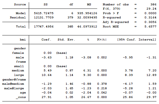
You show this table in your PowerPoint presentation because you know your audience is expecting some statistics, though they don’t really understand them. You begin by explaining that the constant (_cons) represents the mean BMI of small frame women. You have now lost half of your audience because they have no idea why the constant represents small frame women.
By the time you start explaining the interaction you have lost 95% of your audience. You realize that this approach was a bad idea. Would there have been a better way to present these results?
First rule, always know your audience. How statistically knowledgeable are they? What are they interested in knowing?
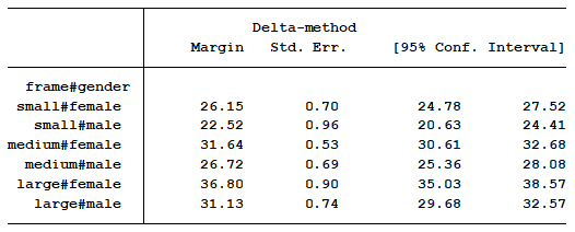
My approach would have been to start by showing them the marginal means for each of the six groups. This table is easy to understand and to interpret. This is not the default output from the statistical software, but it’s not hard to obtain.
Note that I excluded the t-score and p-values. That information is not important because it tells us whether the marginal mean of each category is significantly different from zero.
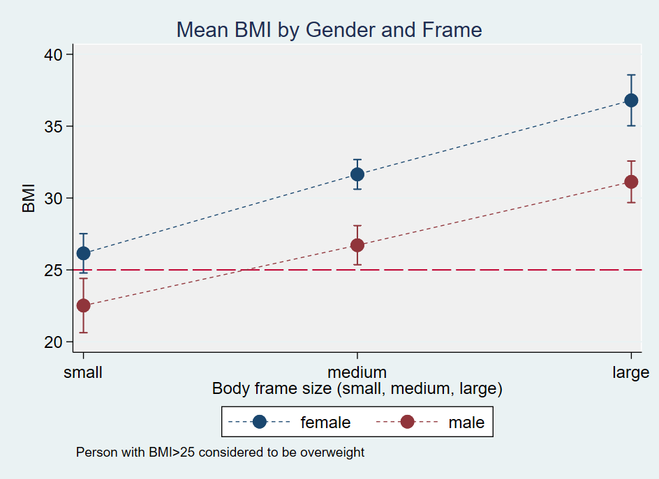
I would then graph the marginal means because it’s easier to visualize the results.
As a finale, I would then address the question the dieticians all had. Are there differences among the six groups? I answer that question by running a pairwise comparison.
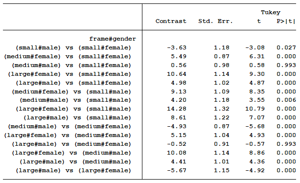
I can now easily explain to them that there is a statistical difference between every combination of sex and gender with regards to mean BMI except for two situations.
Furthermore, the differences in means for each comparison clearly communicates the size of each effect. For example, we can see the size of the gender effect is -3.63 for people with small frames, -4.93 for people with medium frames, and -5.67 for people with large frames.
You know and can report that these contrasts are not significantly different from each other because that is what the interaction terms in your original regression model measured. You can have that information ready for any members of the audience who are interested in that specific test and who will understand the output. (Appendices are a great place for this).
No one is left scratching their head.
While this example showed a linear model, this exact approach is especially useful for understanding the effects of categorical variables with interactions in generalized linear models. In that situation, though, you have to make sure you’re not using p-values on marginal means that have been back-transformed.
Jeff Meyer is a statistical consultant with The Analysis Factor, a stats mentor for Statistically Speaking membership, and a workshop instructor. Read more about Jeff here.

“In that situation, though, you have to make sure you’re not using p-values on marginal means that have been back-transformed.“
Can you please further elaborate on what you exactly mean here, or can you provide links that further illustrate this? I am working on a logistics model of 3#8 interaction level variables and this will help me make sure of using correct estimates to display my results when it comes to using predicted margins.
Hi Muwada,
What we are saying here is the p-value only holds true if you are interpreting the output as it is generated within the model. For example, if you transformed a predict and want to back transform it to its original state, the p-value is not reliable. If you don’t transform the predictor then that is not an issue that you have to consider.
Jeff
Let me add that we can always re-grid the marginal means to the response scale and perform all calculation on the new grid. Typical case: logistic regression: by default all hypotheses are tested on the log-odds scale, which is the linear predictor scale. But this says nothing about comparing probabilities, which is often of interest. Yes, we can transform, do hypothesis testing and back-transform, but the reliability of p will be compromised, as you said, so we result in a difficult to interpret ratios. Definitely not the difference in probability we wanted. So we can make the predictions on the probability scale and construct comparisons directly on this scale, so no need to back-transform anything. We obtain both CIs and p-values on the probability scale. The only problem is that for Wald’s inference these are symmetric, so near to 0 or 1 we may end up with CIs 1. In this case it’s better to use the linear predictor scale to avoid that issue. We could also use likelihood ratio test, which is transformation invariant, unlike Wald’s, so we don’t need to think about the scale, just check the change in deviance when the comparison is performed.
Hello,
Thanks for this incredibly clear explanation. I ran a similar analysis, and got what I think is some odd output. Some of the values of my significance tests P>[t] are -0.000. Is this troublesome? I’m not sure how to interpret this! Any advice?
Thank you again!
Hi,
It’s possible to have a negative Z-score but I have never seen a negative p-value. P-values are between 0 and 1.
Hello,
First of all, thank you for this article, it is really helpful to understand how to interpret the interactions. I followed your instructions and when I ran the Stata code, it tells me that “method tukey is not allowed with results using vce(robust)”. Therefore, I just ran the code pwcompare i.variable1#i.variable2, pveffects, and it worked, but I am not quite sure whether it makes sense this way. What difference exists between my code and yours?
Thank you a lot,
Lola
Hi Lola,
There are some post estimation commands you cannot run if you use “robust” in your model (which I recommend you always include). I rerun my models without the robust to run those post estimation commands. The robust variance doesn’t play a role in calculating the pairwise differences. That being said, using the margins command and including pwcompare will give you similar results to just using the pwcompare command.
Jeff
May I have your Stata Syntax (code) for the examples you explained in this blog and in your webinar?
Thank you very much,
van
Hi Van,
Here is the code for the model:
reg bmi i.gender##i.frame age , cformat(%6.2fc) base
For the marginal means:
margins gender#frame, cformat (%6.2fc) nopvalues
For the graph:
marginsplot, title(Mean BMI by Gender and Frame) ytitle(BMI) ylabel(,angle(horizontal)) yline(25, lpattern(longdash)) ///
plotregion(fcolor(gs15)) plotopts(lwidth(none) msize(large)) note(Person with BMI>25 considered to be overweight)
For the pairwise comparison:
pwcompare frame#gender, mcomp(tukey) pveffects cformat (%6.2fc)
Jeff