At times it is necessary to convert a continuous predictor into a categorical predictor. For example, income per household is shown below.
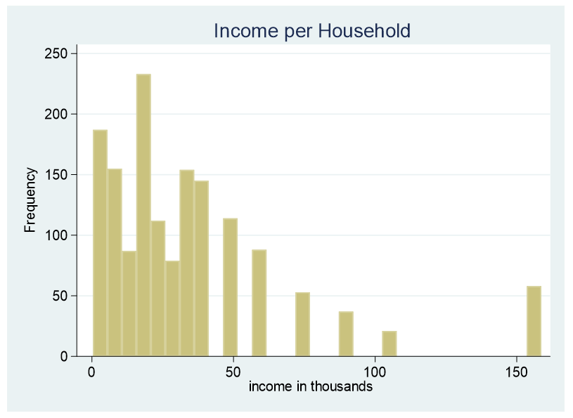
This data is censored, all family income above $155,000 is stated as $155,000. A further explanation about censored and truncated data can be found here. It would be incorrect to use this variable as a continuous predictor due to its censoring.
This does not mean this data cannot be used as a predictor. The data can be converted into a categorical variable. How can we determine the number of categories and the increments of income that are in each category?
The first question to ask: is the analysis theory driven or exploratory? If it is theory driven the break points should take into consideration findings from the literature.
If the analysis is exploratory, the following is one method that can be used for determining break points.
The number and the increments of the categories are determined by the dependent variable. We want groups that are statistically different from each other in relationship to the dependent variable. We can begin this process by graphing.
Below is a scatter plot of household income on the X axis and the dependent variable, Occupational Prestige Score, on the Y axis. Included is a LOWESS curve.
LOWESS is an acronym for “locally weighted scatterplot smoothing.” A LOWESS curve is the result of a moving average and polynomial regression.
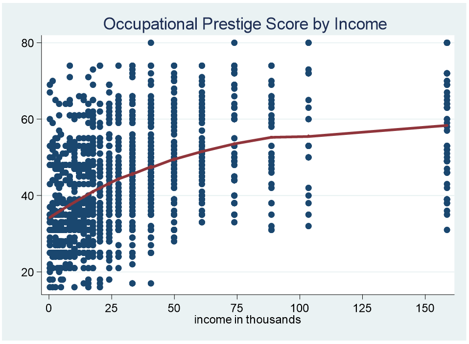
Notice that it is a curve and not a straight line which allows us to look for parts of the curve that are consistent across a specific range. For example, the curve from 100 to 155 is flat. The curve from zero to 15k is similar.
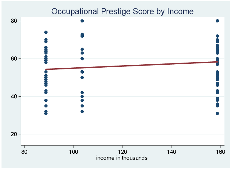
We can then graph the different increments to see how consistent the data is across its range. This time we are going to use the linear best fit line rather than the LOWESS curve. If the best fit line is flat we can deduce that the data is consistent across the range.
Here is the graph for family income greater than $100k.
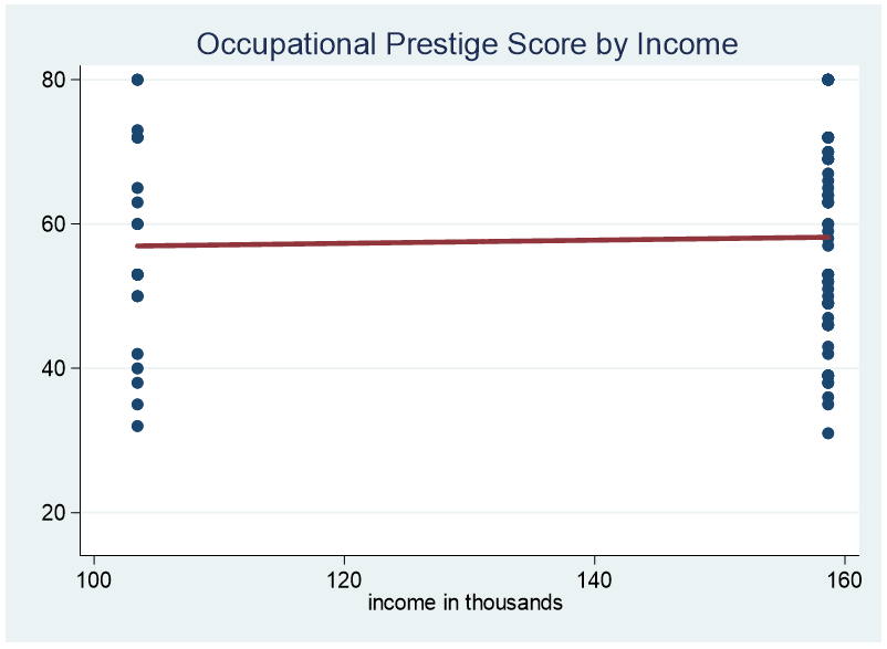
It might be possible to extend the range from $80k to $155k.
Here is an example of the range from $25k to $35k.
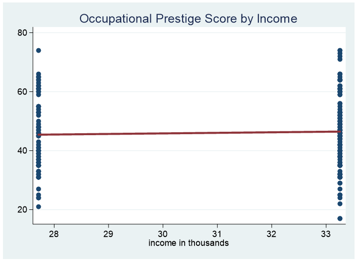
After determining our “best guess” for the various categories we can run pairwise comparison tests of adjacent categories to determine whether the categories are significantly different. If two adjacent categories are not statistically significant it is advisable to combine the categories.
Jeff Meyer is a statistical consultant with The Analysis Factor, a stats mentor for Statistically Speaking membership, and a workshop instructor. Read more about Jeff here.
Leave a Reply