by Jeff Meyer
As mentioned in a previous post, there is a significant difference between truncated and censored data.
Truncated data eliminates observations from an analysis based on a maximum and/or minimum value for a variable.
Censored data has limits on the maximum and/or minimum value for a variable but includes all observations in the analysis.
As a result, the models for analysis of these data are different. (more…)
Most of the p-values we calculate are based on an assumption that our test statistic meets some distribution. Common examples include t distributions, F distributions, 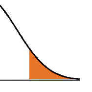 and chi-square distributions.
These distributions are generally a good way to calculate p-values as long as assumptions are met.
But it’s not the only way to calculate a p-value.
Rather than come up with a theoretical probability based on a distribution, exact tests calculate a p-value empirically.
The simplest (and most common) exact test is a Fisher’s exact for a 2×2 table.
Remember calculating empirical probabilities from your intro stats course? All those red and white balls in urns? (more…)
How do you choose between Poisson and negative binomial models for discrete count outcomes?
One key criterion is the relative value of the variance to the mean after accounting for the effect of the predictors. A previous article discussed the concept of a variance that is larger than the model assumes: overdispersion.
(Underdispersion is also possible, but much less common).
There are two ways to check for overdispersion: (more…)
 As mixed models are becoming more widespread, there is a lot of confusion about when to use these more flexible but complicated models and when to use the much simpler and easier-to-understand repeated measures ANOVA.
One thing that makes the decision harder is sometimes the results are exactly the same from the two models and sometimes the results are (more…)
One of the many confusing issues in statistics is the confusion between Principal Component Analysis (PCA) and Factor Analysis (FA).
They are very similar in many ways, so it’s not hard to see why they’re so often confused. They appear to be different varieties of the same analysis rather than two different methods. Yet there is a fundamental difference between them that has huge effects on how to use them.
(Like donkeys and zebras. They seem to differ only by color until you try to ride one).
Both are data reduction techniques—they allow you to capture the variance in variables in a smaller set.
Both are usually run in stat software using the same procedure, and the output looks pretty much the same.
The steps you take to run them are the same—extraction, interpretation, rotation, choosing the number of factors or components.
Despite all these similarities, there is a fundamental difference between them: PCA is a linear combination of variables; Factor Analysis is a measurement model of a latent variable.
Principal Component Analysis
PCA’s approach to data reduction is to create one or more index variables from a larger set of measured variables. It does this using a linear combination (basically a weighted average) of a set of variables. The created index variables are called components.
The whole point of the PCA is to figure out how to do this in an optimal way: the optimal number of components, the optimal choice of measured variables for each component, and the optimal weights.
The picture below shows what a PCA is doing to combine 4 measured (Y) variables into a single component, C. You can see from the direction of the arrows that the Y variables contribute to the component variable. The weights allow this combination to emphasize some Y variables more than others.
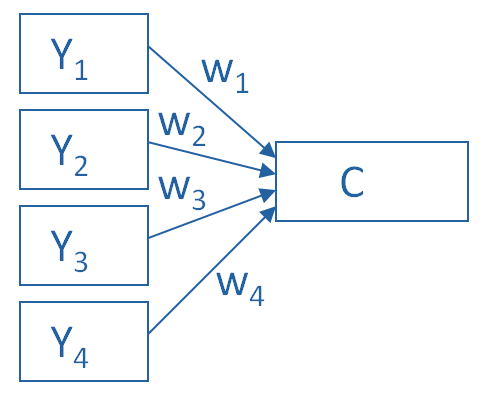
This model can be set up as a simple equation:
C = w1(Y1) + w2(Y2) + w3(Y3) + w4(Y4)
Factor Analysis
A Factor Analysis approaches data reduction in a fundamentally different way. It is a model of the measurement of a latent variable. This latent variable cannot be directly measured with a single variable (think: intelligence, social anxiety, soil health). Instead, it is seen through the relationships it causes in a set of Y variables.
For example, we may not be able to directly measure social anxiety. But we can measure whether social anxiety is high or low with a set of variables like “I am uncomfortable in large groups” and “I get nervous talking with strangers.” People with high social anxiety will give similar high responses to these variables because of their high social anxiety. Likewise, people with low social anxiety will give similar low responses to these variables because of their low social anxiety.
The measurement model for a simple, one-factor model looks like the diagram below. It’s counter intuitive, but F, the latent Factor, is causing the responses on the four measured Y variables. So the arrows go in the opposite direction from PCA. Just like in PCA, the relationships between F and each Y are weighted, and the factor analysis is figuring out the optimal weights.
In this model we have is a set of error terms. These are designated by the u’s. This is the variance in each Y that is unexplained by the factor.
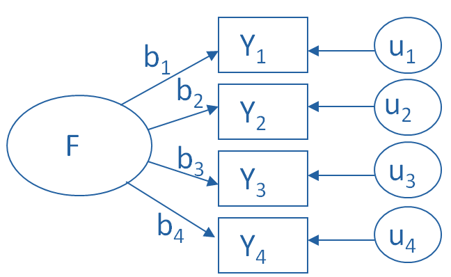
You can literally interpret this model as a set of regression equations:
Y1 = b1*F + u1
Y2 = b2*F + u2
Y3 = b3*F + u3
Y4 = b4*F + u4
As you can probably guess, this fundamental difference has many, many implications. These are important to understand if you’re ever deciding which approach to use in a specific situation.
Go to the next article or see the full series on Easy-to-Confuse Statistical Concepts
Despite modern concerns about how to handle big data, there persists an age-old question: What can we do with small samples?
Sometimes small sample sizes are planned and expected. Sometimes not. For example, the cost, ethical, and logistical realities of animal experiments often lead to samples of fewer than 10 animals.
Other times, a solid sample size is intended based on a priori power calculations. Yet recruitment difficulties or logistical problems lead to a much smaller sample. In this webinar, we will discuss methods for analyzing small samples. Special focus will be on the case of unplanned small sample sizes and the issues and strategies to consider.
Note: This training is an exclusive benefit to members of the Statistically Speaking Membership Program and part of the Stat’s Amore Trainings Series. Each Stat’s Amore Training is approximately 90 minutes long.
(more…)